This document discusses the details of using the DIRSIG image and data generation model to simulate laser remote sensing systems.
The terms LIDAR (or LiDAR) and LADAR are generally used interchangeably and numerous articles have been written about what types of applications are LIDAR vs. LADAR. If you hunt for the differences, you will eventually find that there is some consensus that these two terms are uniquely mapped to two distinct types of systems. Laser Detection and Ranging (LADAR) is the term that is most appropriately used with a laser system that attempts to measure the distances (ranges) to hard objects including the ground or other target objects by computing the time of flight for a pulse to leave the transmitter, reflect off the object and return to the receiver. This timing can be accomplished with both incoherent and coherent detection schemes. Light Detection and Ranging (LIDAR or LiDAR) is sometimes considered a more generic term, but is also associated with systems that attempt to characterize the optical properties of diffuse or volumetric objects. For example, atmospheric aerosols are typically measured by computing the absorption (due to scattering) of a laser pulse over a path of known distance. Differential Absorption LIDAR (DIAL) systems attempt to characterize the concentration of gases in the the atmosphere by comparing the relative absorption of a laser pulse at a pair of wavelengths (one where the gas doesn’t have much absorption and one where it does).
So although there is some agreement that there are unique application areas for LIDAR and LADAR, it appears to be generally acceptable these days to use the two terms interchangeably.
Overview
The DIRSIG model includes an active laser-sensing (LIDAR) model that utilizes a unique particle-oriented approach to beam propagation and surface interaction. This approach has been shown to be radiometrically accurate and it can predict a variety of important geometric effects including multiple-bounce (multiple-scattering) effects. [1]. We believe that the DIRSIG model’s capability for simulating lidar data is unique and includes a higher level of fidelity than any other known modeling tool. Many tools simulate lidar by taking a DEM and computing an area-wide reflected intensity based on simplified source and receiver geometry and surface optical properties. That intensity field is then degraded with image processing techniques to model effects like scintillation and speckle.
The DIRSIG model simulates the propagation of the source pulse into the scene, how it interacts with the 3D scene and propagates it back to the receiver. This rigorous radiometric prediction is then coupled with detailed detection models and product generation tools to generate a variety of low-level data products including geolocated 3D point clouds or 2D detection maps.
|
|
An Advanced Geiger-mode APD Detector Model was made available in DIRSIG 4.7. The advanced tool focuses on modeling specific aspects of GmAPD systems and requires a great deal of engineering data (that is not generally available) in order to be used effectively. For most users, the basic GmAPD model described in this document is sufficient. |
Technical Readiness
This application area is currently ranked as mature. The discussion below lists additional features and capabilities that can still be addressed.
Model Strengths
-
Model driven (e.g. MODTRAN, MonoRTM, etc.) atmospheric absorption and scattering
-
Atmospheric refraction (bent path) and non-uniform speed of light effects can be incorporated via data-driven temperature, pressure and relative humidity profiles.
-
-
Usage of the same detailed surface and volume optical descriptions employed in passive simulations
-
A suite of mono-directional reflectance distribution (MRDF) and bi-directional reflectance distribution (BRDF) models, including those with support for polarization.
-
Scattering and absorption from participating mediums (clouds, water, fogs, etc.)
-
-
Complex scene geometries for arbitrary polygon defined terrains and scene objects (natural and man-made)
-
Scene objects can move as a function of time, resulting in pulse-to-pulse displacement and Doppler shifting effects
-
-
Usage of the same platform motion and platform-relative scanning models employed in passive simulations.
-
The platform motion and platform-relative scanning models support temporally uncorrelated (mean and standard deviation) and temporally correlated (magnitude and phase frequency spectrum) jitter.
-
Platform-relative mounting and scanning allows for both mono-static and bi-static configurations.
-
-
Inclusion of passive (background) photons
-
Multiple bounce/scattering through a modification to a numerical approach called "Photon Mapping" (discussed in more detail later in this document)
-
Pulse-to-pulse cross-talk when multiple pulses are in flight from high-altitude and/or high pulse repetition rate systems
-
User-defined range gate (listening windows), including dynamic range gate options (command data driven)
-
The ability to specify transmit and receive path polarization on a pulse-to-pulse basis (command data driven)
-
Support for a variety of detection architectures including linear mode, Geiger mode, photon counting and waveform
-
Support for knowledge errors in the generation of Level-1 point clouds
Model Weaknesses
-
The beam propagation is strictly geometric at this time.
-
A plug-in interface has been developed to allow wave-based models to handle the propagation of the beam from the exit aperture to the scene. This allows turbulence induced beam spread, wander and scintillation to be incorporated into the simulation. However, the one plug-in that has been developed against that interface it not available to the general user community at this time and documentation of the plug-in API has not been completed to allow other 3rd parties to develop against it.
-
-
The radiometry engine and detection models are focused on incoherent detection systems at this time.
-
RADAR simulations in DIRSIG do handle strict phase tracking to support systems requiring coherence, including Synthetic Aperture RADAR (SAR) systems. We believe it would be possible for those approaches to be adapted to the LIDAR related radiometry solutions.
-
-
The Direct+PM radiometry approach does not currently support speckle (either fully or partially developed) at this time.
-
Early prototypes of the DIRSIG model did include a fully developed speckle solution, but the production code has been focused on systems that are not speckle-limited. Therefore, the inclusion of speckle modeling has not been a priority.
-
-
The Linear-mode APD detector model does not currently include noise
-
An accepted model for modeling Level-0 noise induced errors is not available at this time, primarily due to the proprietary nature of commercial Linear-mode system trade craft.
-
-
Output of Level-0 (raw time-of-flight) data is not supported at this time.
-
This data exists within the detector model module, however a well accepted format for Level-0 data does not appear to exist.
-
The existence of these limitation is primarily a result of funded research priorities. Our past and current research has not placed a priority on resolving this current set of limitations. As researchers, we are always seeking opportunities to to address known limitations if funding is available.
Two Stage Simulation Approach
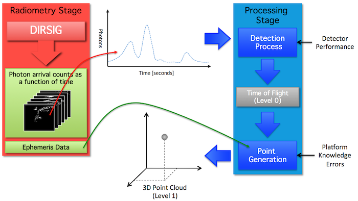
To maximize the flexibility in modeling end-to-end LIDAR systems, a full simulation is divided into two, discrete stages. Stage 1 is the "Radiometric Simulation" that (for each pulse) computes the temporal flux received by each pixel during a user-specified listening window. That result is then input into Stage 2, or the "Detector Model and Product Generation" stage, where the output of Stage 1 is coupled with a separate, back-end detection model to convert the temporal photon arrival times into common data products (e.g. geo-located point clouds).
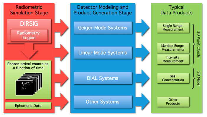
The "Detector Modeling and Product Generation" tool models (a) the unique characteristics of the detector type employed in the receiver to generate time-of-flight measurements and (b) converts those time-of-flight measurements into 3D points within a 3D point cloud (see the figure below). The DIRSIG model is distributed with multi-return Linear-Mode (Lm), single-return Geiger-Mode (Gm) and multi-return photomultiplier tube (PMT) detector models that will be discussed in the later sections of this document.
|
|
In the event that the standard detector models provided with DIRSIG do not suite your needs, it should be noted that the creation of custom detector model and product generation tools has been accomplished by several members of the DIRSIG user community. Although guidelines for doing this are not presented here, the key is to parse the radiometric output of the DIRSIG Radiometric Simulation (the BIN file) and implement your own time-of-flight measurement modeling and point generation procedures. |
This two-stage approach provides a lot of flexibility for doing detector performance studies because the detection and product generation can be repeatedly performed very rapidly once the intermediate radiometric data product has computed. The details of these two stages are discussed in later sections of this document.
System Description
At the heart of a DIRSIG LIDAR simulation is a flexible and detailed description of the acquisition platform. Like the passive systems modeled with DIRSIG, an active system can be placed at a fixed location (for example, a tripod) or on a moving platform (for example, a ground vehicle, aircraft or spacecraft). The details of platform positioning are beyond the scope of this document. Instead this document will attempt to describe the detailed transmitter and receiver characteristics available to the user. These include (but are not limited to):
-
System Characteristics
-
User-defined platform location and orientation (altitude, speed, etc.). See the Platform Position Data guide for more information.
-
Platform relative scanning using built-in periodic scanning mounts (whisk, lemniscate, etc.) or user-defined scanning using measured platform-relative pointing angles. See the Instrument Mounts guide for more information.
-
-
Source Characteristics
-
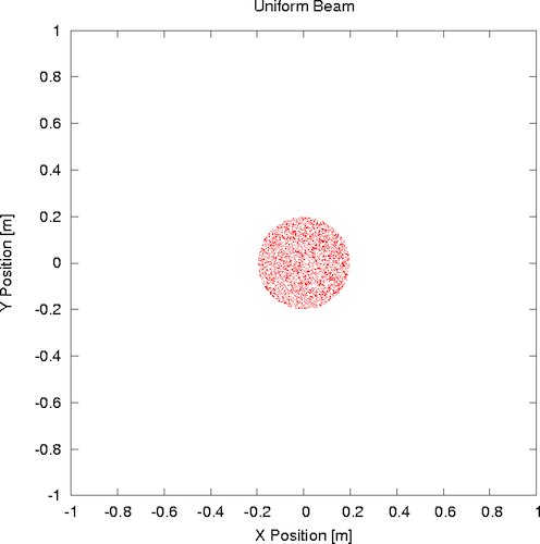
Spatial (transverse) beam profile using either functional forms (Gaussian, Sinc, etc.) or a user-defined 2D intensity profile ("burn paper").
-
Spectral shape using functional forms (Gaussian, Lorentzian, etc.).
-
Pulse energy and temporal pulse profile using either functional forms (Gaussian, etc.) or a user-defined 1D profile.
-
User-defined stable pulse repetition rate (PRF) or user-defined shot times.
-
Support for fixed or dynamic polarization state generator (PSG).
-
-
Receiver Characteristics
-
User-defined focal length, aperture size and optical throughput.
-
User-defined number of receiver focal plane arrays (FPAs).
-
Each FPA can have unique:
-
Numbers of pixels, pixel size and pixel spacing.
-
Relative spectral response functions using either functional forms or a measured response function.
-
Support for fixed or dynamic polarization state analyzers (PSAs).
-
-
Radiometric Simulation Stage
DIRSIG4 Approach
The addition of an active, laser radar capability to the DIRSIG4 model was accomplished by the addition of a suite of new objects to the existing radiometry framework. In general, the model is designed to predict the returned fluxes from the scene as a function of time with respect to the shooting of the source laser. The specific challenges of this imaging model were driven by the requirement to predict the received photon counts as a function of space and time. The photon flux arriving at a LIDAR system often approaches discrete photon events due to the low amount of backscattered radiation and can prove difficult for many traditional Monte-Carlo ray tracing techniques. Additionally, the temporal structure of these returns is driven by the spatial structure of the scene and the total travel time of arriving photons accrued during multiple bounce and scattering events within the scene. Analytical, statistical, and existing passive radiometry solvers were found to be insufficient in many instances, particularly for low flux situations. Thus, a new approach was sought.
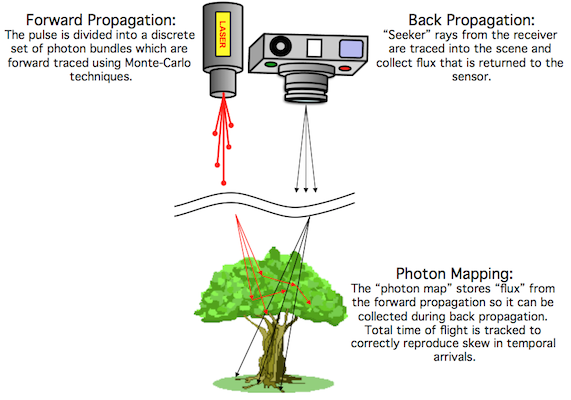
We hybrid approach we implemented is called "Direct Return and Photon Mapping" or "Direct+PM", for short. This hybrid approach leverages a modeling technique called "photon mapping" (Jensen, 2001). [2]. The "direct return" aspect entails backward ray-tracing from the receiver focal plane(s) into the scene. At each intersection, a direct (single bounce) contribution is computed by ray tracing to the transmitter (source). This calculation incorporates surface and/or volume optical properties and the characteristics of the source (spatial/angular intensity, etc.).
The multiple bounce (or multiple scattering) contribution for the location employs a modification to the photon mapping approach. One reason that this technique was selected was because photon mapping has been demonstrated to be applicable to traditional solid geometry reflective illumination and scattering and absorption by participating mediums, particularly in multiple bounce and multiple scattering cases. The photon mapping approach is a hybrid of traditional forward and backward Monte-Carlo ray tracing techniques. In this two-pass method, source photon "bundles" (a set of literal photons that are assumed to travel together) are shot from a source into the scene using forward ray tracing during the first pass and then collected using a backward ray tracing during the second pass. The collection or rendering process utilizes the events recorded during the first pass to calculate the sensor reaching radiance. For the purpose of active laser radar applications, some modifications to the basic photon mapping treatment were made including the tracking of total travel time and a literal photon counting process.
Model Approach
During the first pass, a modeled "photon bundle" is shot into the scene from the source and performs a pseudo-random walk through the scene based on the optical properties of the surfaces or mediums that it encounters. At the location of each interaction, information regarding the interaction event is stored into a fast, 3D data structure or map (e.g. a kd-tree) that can be queried during the second pass. A critical addition to traditional photon mapping paradigm was a field to track each photon’s total travel time. This time field accrues the travel time for all of the multiple bounce/scattering events to be recorded and is used for time gating during the second pass. The modeled "photon bundle" is followed until it is absorbed by some element within the scene. The photon casting process is repeated until a specified number of interaction events have been recorded in the map. The characteristics of the laser source are incorporated into the spatial, spectral and temporal distribution of the modeled photon bundles fired into the scene.
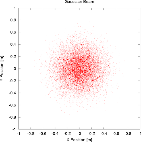
Like the surface reflectance and volume scattering processes, the shooting of the photon bundles employs importance sampling. In this case, more photon bundles are emitted from the source into directions where the intensity of the source is higher (see the example plots of shot photon bundles below).
The numerical error of the estimated received photon stream is intimately linked to the number of "photon bundles" cast into the scene. The number cast must be sufficient to obtain a statistically significant number of events throughout the field-of-view of the sensor. Depending on the angular extent of the beam, the field-of-view of the sensor and the spatial detail of the scene approximately 250,000 to 1,000,000 "photon bundles" can be utilized in the photon mapping process to create reliable statistics for topographic returns. For volume scattering returns, this number may need to be higher depending on the absorption and scattering coefficients and the spatial extent of the participating volumes.
For the second pass, rays are shot from the image plane into the scene until a scene element is intersected. Traditional photon mapping approaches utilize the localized photon map density to estimate the incident irradiance at a surface or volume element. The radiometry algorithm queries the 3D data structure that was filled during the first pass to find a set of incident "photon bundles" arriving at the surface (or volume element in the case of a participating medium). The volume over which the photons are collected is based upon the detector’s field-of-view and a user-defined spatial oversampling factor. Each of these "photon bundles" is individually redirected towards the sensor using the applicable surface reflectance or volume scattering coefficients for the specific incident and exitant geometry. This redirection simply computes the fraction of real photons in the bundle that would be reflected or scattered toward the receiver. The received photons are then temporally distributed (based on the bundle’s parametric temporal shape) and quantized based upon the user-defined listening window and sampling frequency. The result is a time-gated data cube for the listening window that contains the received number of photons at each sampling interval for each detector element.
Model Implementation
The integration of photon mapping into the DIRSIG model entailed the implementation of several new objects. The first was the basic support for photon mapping. This entailed the implementation of a 3D data structure that can be quickly searched using spatial queries and the creation of a photon object that would be propagated and stored into the photon map. For this purpose, the traditional kd-tree was used. The next object was a flexible source model that could support directional characteristics and the spatial, spectral and temporal distribution of the source photons. In the current implementation, the system is modeled in a monochromatic mode at the peak wavelength of the source and the spectral width is stored parametrically, rather than shooting photons as a function of wavelength. The temporal shape of the pulse is stored parametrically in each "photon bundle" rather than shooting photons as a function of time. The pointing and spatial (transverse) beam profile of the source is numerically driven by either analytical or data-driven 2D profiles. The LIDAR support allows the user to model co-axial and bi-static systems by providing nearly arbitrary relative source to detector positioning and pointing geometries.
The photon shooting function leverages the generic ray tracing support that already existed within the DIRSIG model. The ray tracer interacts with scene elements that have material specific properties. Each material has a set of surface optical properties and an optional set of bulk or medium properties. The surface properties include a spectral reflectance and/or emissivity property. The currently supported reflectance (BRDF) models include importance based sampling functions to support the forward and backward Monte-Carlo ray tracing. The bulk properties include spectral extinction, absorption and scattering coefficient models. When volume scattering is modeled, a phase function object can also be configured to describe the directional nature of the scattering. The phase function objects also support importance based sampling functions to support the forward and backward Monte-Carlo ray tracing. Although these optical descriptions existed prior to the addition of the LIDAR capabilities, their interfaces were enhanced during this effort to facilitate an efficient implementation of the photon mapping subsystem.
The next major component of the model to be implemented was the collection of photons from the photon map and forward propagation into the imaging system. The modeling of the radiometric returns from a scene element is handled by a class of objects in DIRSIG referred to as radiometry solvers. A radiometry solver encapsulates an approach to predicting the energy reflected, scattered and emitted by a surface or volume. For example, there already existed a specific solver for predicting the passive returns from "hard" surfaces and another for a volume of gas (e.g. plume). These solvers utilize the material specific surface and bulk optical properties to predict their results. One or more radiometry solvers can be assigned to each element in the scene. To support the active LIDAR returns, a new radiometry solver was created to compute the returns from a scene surface or volume by using the optical properties and the photon map to estimate the number of incident photons at the element’s point in space. Unlike the existing passive radiometry solvers that would place the final result in a time-independent result object, the LIDAR-specific radiometry solver places the result into a time-gated result object. The time gating is based on a user-defined signal gate consisting of a start, stop and delta time. The final component was the implementation of a "capture method" object within the system that directs how outputs for the detectors on the focal plane are computed. The LIDAR specific capture method developed under this effort backward propagates rays from each detector element into the scene where it intersects scene elements, runs the appropriate radiometry solvers (passive and active), forward propagates the energy to the focal plane and then writes the arriving photons counts to the output file.
DIRSIG5 Approach
The issue with the photon mapping approach used in DIRSIG4 was that the user was required to correctly setup key parameters for the algorithm to work correcly. Incorrect configuration of the photon mapping parameters could yield incorrect link budgets, noisy returns, etc. One of the overarching goals of DIRSIG5 was to eliminate the dependence on the user correctly configuring the complex algorithms used by the radiometry solvers, photon mapping, etc. Hence, In DIRSIG5, the radiometry core was united under the path tracing numerical radiometry method that provides the user with a single variable to control the radiometric fidelity (how many samples or paths per pixel). DIRSIG5 still incorporates a bi-directional propagation approach but it is fully automated and does not require user configuration. The DIRSIG5 approach models the laser pulse as a geometric mesh that can be propagated, distorted, refracted, etc. The path tracing method can query these pulses and incorporate the energy into the solution.
Important Change in DIRSIG5
There is an important difference between DIRSIG4 and DIRSIG5 that should be noted because it uniquely impacts LIDAR simulations. In DIRSIG5, one of the not so apparent differences in the radiometry engine is that it is sampling the spectral dimension. This was a decision made early on in the DIRSIG5 design to make things more consistent across the “big three” dimensions (spatial, spectral and temporal). We are clearly spatially sampling (with rays) and temporally sampling (with ray times) the world, and now the spectral dimension is treated similarly.
The important change is that in DIRSIG4, the transmitter (laser) spectral line shape was "rendered" into the spectral dimension using spectral integrals. Hence, if your transmitter (laser) spectral line width was much narrower than the receiver spectral bandpass, all the spectral energy would have been integrated into the spectral bin containing the line. However in DIRSIG5, the line is being sampled by the spectral bins. As a result, if your receiver bandpass sampling is much coarser than the transmitter spectral line width, a portion or even all of the transmitter energy can be lost.
To model this correctly, the spectral sampling used in the radiometry core should effectively sample the transmitter (laser) spectral line shape. In terms of user inputs, the receiver spectral bandpass should be a sufficiently high resolution compared to the line width. When the DIRSIG5 BasicPlatform initializes it will check this sampling and issue a warning or even a fatal error if the sampling is found to be inadequate.
Initializing the 'BasicPlatform' plugin
Initializing 'Demo APD Ladar'
    Using convergence parameters = 50, 100, 1.000e-12,
    Using a maximum of 4 nodes per path
[warning] Receiver bandpass delta is not << than the transmitter line width!
[warning] This can/will result in an inaccurate link budget!Initializing the 'BasicPlatform' plugin
Initializing 'Demo APD Ladar'
Using convergence parameters = 50, 100, 1.000e-12,
Using a maximum of 4 nodes per path
[error] while initializing an instrument:
LidarInstrument::init: Receiver bandpass delta >= Transmitter line width!
[error] Simulation ended unexpectedly with error:|
|
This check cannot be performed for bi-static and multi-static setups since the transmitter(s) and receiver(s) are contained in separate objects and cannot be compared. |
Radiometric Data Product
The DIRSIG model outputs a radiometric product defining the number of photons incident on pixel, for each FPA, for each pulse. This radiometric data product is essentially a set of spatial x spatial x temporal (waveform) cubes (one 3D cube for each pulse). A complete description of this radiometric product is described in the BIN file documentation.
BIN File Analysis
The contents of a BIN file can be quickly summarized
by an analysis tool that is included with DIRSIG. This tool can be
accessed on the command-line as the program bin_analyze or via
the Detector Model graphical user interface via the Analyze
button on the Input tab.
The program will print out the contents of the various headers in the BIN file and will include basic statistics for each pulse. Example output of a BIN file containing a single pulse that was created with a single pixel receiver is shown below:
$ bin_analyze example.bin

File Header:
    Created: 201209061918.17
    DIRSIG Version: 4.5.0 (r11191)
    File Version: 1
    Scene Origin: 43.12 [+N], -78.45 [+W]
    Scene Altitude: 300 [m]
    Source Mount: Unknown Mount
    Receiver Mount: Unknown Mount
    Focal Plane Array ID: 0
    Array Dimensions: 1 x 1 pixels
    Pixel Count: 500 x 500 [microns]
    Lens Distortion Coeffs: 0 , 0
    Task Count: 1

Task Header:
    Start Date/Time: 200906010000.00
    Stop Date/Time: 200906010000.00
    Focal Length: 400 [mm]
    Pulse Rate: 2000 [Hz]
    Pulse Duration: 5e-09 [s]
    Pulse Energy: 1e-05 [J]
    Laser Line: 1.064 [um]
    Laser Width: 0.0003 [um]
    Pulse Count: 1

Analyzing pulse #1
Pulse Header:
    Pulse time: 0
    Time Gate Open: 1.2e-05 [s], 1798.75 [m]
    Time Gate Close: 1.4e-05 [s], 2098.55 [m]
    Time Bin Count: 2001
    Samples Per Time Bin: 1
    Contains compressed pulse data
Pulse #1:
    Minimum total photons in a pixel = 12.86
    Maximum total photons in a pixel = 12.86
    Pixels with zero total photons = 0/1 (0%)
    Average total photons per pixel = 12.86

Complete!|
|
Before the 4.5 release, this tool was called proto_analyze.
It was renamed bin_analyze for the 4.5 release to make the
name more intuitive.
|
The bin_analyze tool also has two options that are currently only
accessible via the command-line.
Including --output_profiles=true in the arguments will tell the
tool to generate an ASCII/Text file containing the average return
profile for all the pixels in the array. A separate file will
be generated for each pulse in the BIN file using a naming scheme
of profile_N.txt, where N is the pulse number starting at 0.
The file contains six columns:
-
The bin number (integer bin number starting at
0) -
The time-of-flight for the bin (seconds)
-
The total number of photons (summed across all pixels) for the bin
-
The average number of photons (averaged across all pixels) for the bin
-
The minimum number of photons (in any pixel) for the bin
-
The maximum number of photons (in any pixel) for the bin
The plot below was created from a "profile" for a single pulse for a LIDAR receiver containing a single-pixel array by plotting column #1 vs. column #3. Note that because this was a single-pixel array, column #3 and #4 had the same values.
Including --output_grids=true in the arguments will tell the
tool to generate an ASCII/Text file containing the temporally summed
photons for each pixel in the array. A separate file will be
generated for each pulse in the BIN file using a naming scheme of
pulse_N.txt, where N is the pulse number starting at 0.
The file contains three columns:
-
The X coordinate of the pixel in the array
-
The Y coordinate of the pixel in the array
-
The total number of photons received (summed over all time bins) in that pixel
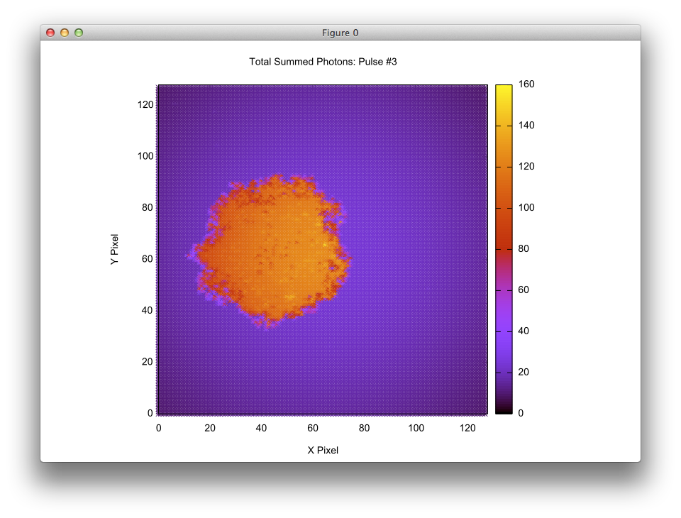
The visualization below was created by plotting an output "grid" file for for a single pulse onto a 128 x 128 pixel array. The data was plotted using the X and Y values (columns #1 and #2) and using the total number of photons (column #3) to drive the color.
Detector Modeling and Product Generation Input
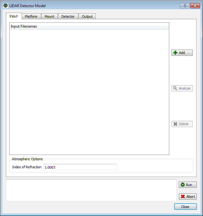
The BIN file produced by the "Radiometric Simulation Stage" is input into the "Detector Modeling and Product Generation Stage" by starting the LIDAR Detector Model from the Lidar Tools sub-menu on the Tools menu. The Input tab allows the user to add one or more input BIN files to the model (multiple BIN files might be produced by a single simulation if separate files are created for each task or each capture (pulse)).
Detector Modeling
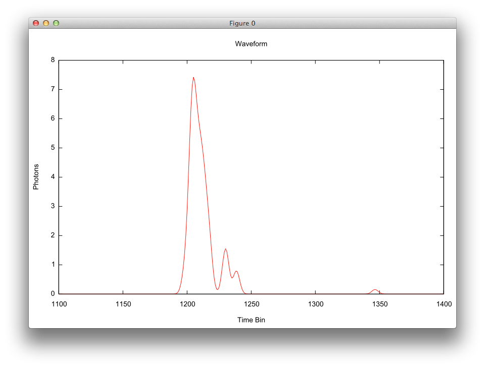
As was described in the previous section, the output of the DIRSIG radiometry simulation is a spatial x spatial x time "cube", where each "pixel" has a time dimension that stores the number of photons in each time bin. In the realm of "Waveform Lidar", these pixel profiles are "waveforms". The image below is plot of a pixel profile looking down on a tree. The X-axis is the time dimension and the Y-axis is the number of photons in each time bin. Note the multi-peak region in the middle that corresponds to the tree (each peak is a different level or branch in the tree) and the small peak near time bin #1350 is a weak return from the ground.
This section will discuss how different detector systems generate returns based on the incident photon flux and the characteristics of the systems.
Linear-Mode Detection
A Linear-mode Avalanche Photo-Diode (LmAPD) device is operated just below the device’s breakdown voltage. Under this operating mode, the device is referred to as a "linear" detector because the generated photocurrent is proportional to the received optical power (it should be noted that this relationship isn’t necessarily perfectly linear at all bias voltages). Generally, LmAPD systems have been employed in higher link budget applications, but as fabrication improvements are made the potential for achieving photon counting sensitivity is increasing.
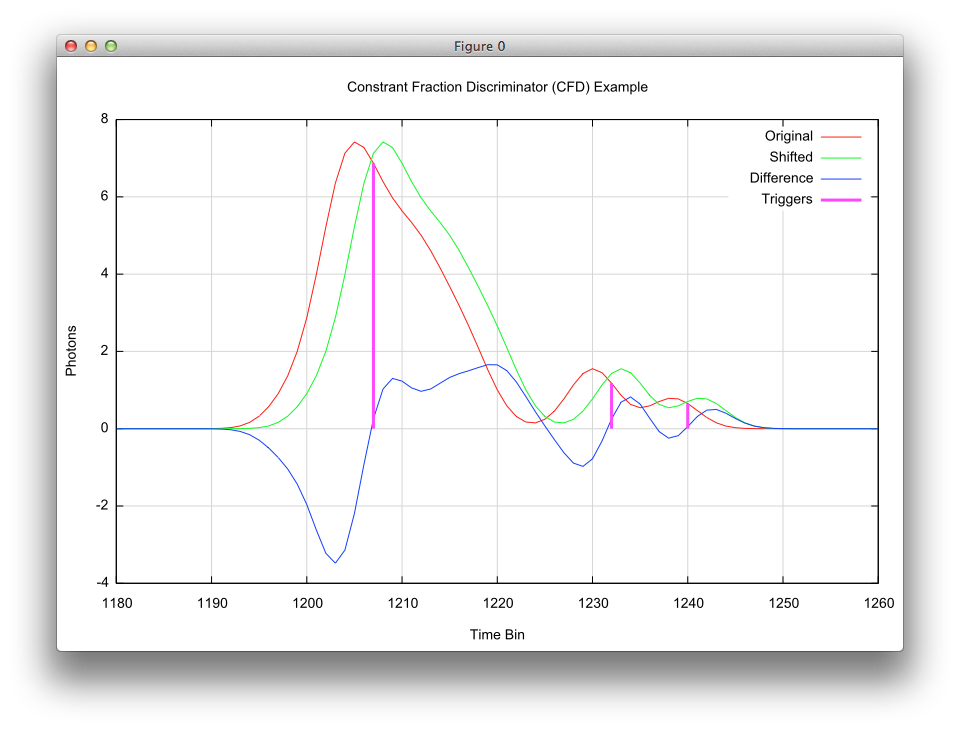
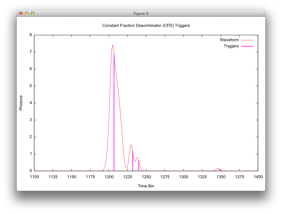
Most Linear-mode (Lm) systems are commercial and as a result specific details about how they work and how they can be modeled isn’t openly published. In practice, the output of an Lm detector is connected to real-time analysis hardware that is "looking" at the signal output as a function of time. The common method used in the real-time analysis is a "constant fraction discriminator" (CFD) rather than a simple threshold. This allows the hardware to detect peaks at various magnitudes.
The linear-mode detection model included with DIRSIG is a basic CFD based detection and timing scheme. The implementation of the CFD in the DIRSIG linear-mode detection model is as follows:
-
Start with the original waveform.
-
A copy of the original waveform is made that is shifted in time.
-
The amount of shift is typically proportional to the pulse width.
-
In real hardware this might be accomplished with some sort of "delay line".
-
-
The difference of the original and shifted waveform is computed.
-
Negative-to-Positive zero crossings in the difference waveform are flagged as trigger times.
-
The magnitude and the time-of-flight are recorded for each trigger.
-
-
Moving forward in travel time, additional triggers that within the "reset time" of a previous trigger are removed.
-
The final set of trigger times (and the corresponding magnitudes) are written to the output file.
-
The user has control over the number of triggers to writing, including if the final trigger should always be included.
-
|
|
At this time noise is not considered in linear-mode detection. This is primarily because we have not found any documented discussion of how noise is characterized in linear-mode systems. |
To illustrate this process, a plot of the these various components are shown below (the X axis has been zoomed to emphasize details). The original received waveform is plotted in red, the shifted waveform is plotted in green and the difference waveform is plotted in blue. The resulting triggers (where the blue difference waveform crosses zero with a positive slope) are plotted as the vertical magenta lines. Note how these trigger lines also capture the magnitude at these trigger times.
|
|
The trigger points in the plot are always located at some "constant fraction" of the pulse width regardless of the magnitude of the peak. |
|
|
The offset of the trigger point relative to the peak is irrelevant because the time-of-flight is computed based on the time elapsed since a trigger from the outgoing pulse. Since that outgoing pulse trigger is at the same fraction (hence, has the same offset), this time shift cancels out. |
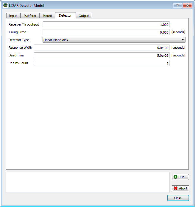
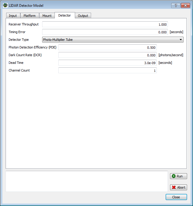
The LmAPD detector model is selected from the Detector Type menu on the Detector tab in the Lidar Detector Model. This provides the interface for the user to set the various parameters describing the detector’s characteristics.
Geiger-Mode Detection
A Geiger-mode Avalanche Photo-Diode (GmAPD) device is a photon counting device that employs a solid state photo-diode that is biased just above the breakdown voltage of the device. A single photo-electron can trigger a breakdown event, generating an avalanche that can directly trigger a timer. However, the device must then be reset after each breakdown event in order to detect a new arrival event, and this process is slow enough that it cannot be accomplished within a single listening window. Hence, the current generation of GmAPD devices can only make a single range measurement per pulse.
The Geiger-mode (Gm) detection model used is an implementation of the model described by O’Brien and Fouche [3]. This approach includes treatment of noise, photoelectron generation and probabilistic detection. The probability of the device firing in bin i is:
\( P(i) = \exp (-fN) [1 -\exp(-S(i) -w)] \)
where f is the fraction of the bins in the range window before the current bin, N is the noise rate per pulse (photoelectron events from passive background flux and dark count across all bins in the listening window), S is the received active signal (in photoelectrons) and w is the noise rate per bin (photoelectron events per bin from passive background flux and dark count). The exp(-fN) term represents the probability that the detector has not been triggered in a previous time bin (remember that a GmAPD device can only trigger once per pulse). The [1-exp(-S(i)-w)] term represents the probability of a trigger in the current time bin due to either signal or noise.
|
|
The photon detection efficiency (PDE) is a combination of the (a) array lenslet transmission, (b) the lenslet to array coupling efficiency and (c) the quantum efficiency (QE) of the GmAPD device itself. If a lenslet array is not employed, then PDE = QE. |
|
|
The dark count rate (DCR) is the rate at which the detector randomly fires due to a variety of noise sources when no photons are incident upon it. |
|
|
Commercially available GmAPD devices report photon detection efficiencies (PDEs) values of 35% and dark count rates (DCRs) of 10 kHz. |
The photon detection efficiency (PDE) and dark count rate (DCR) are incorporated as follows. The signal (S) in photoelectrons is computed from the number arriving photons at the surface of the device multiplied by the PDE. The noise rate per pulse (w) is computed as the dark count rate (DCR) and the background (passive) flux times the length of the listening window (range gate). The noise rate per bin (N) is compute as the noise rate per pulse (w) divided by the number of time bins per listening window.
The equation to compute probability of a trigger in a given time bin can be used to determine at what time the detector will trigger using a Monte-Carlo process. Starting in the first time bin, a random value can be drawn and compared to the probability of that bin. If the random value is lower than the probability, then a trigger occurs in that bin. If not, this process is repeated with the next time bin.
Although this Monte-Carlo approach is correct, it requires a random number to be generated for every time bin. An alternative method is to compute cumulative probabilities across time bins and then draw a single random value to determine during which time bin the detector will fire in. This approach is more attractive computationally because a significantly smaller number of random numbers need to be generated.
The modeling technique cumulative probability approach is as follows:
-
The probabilities (PDF) for each time bin are computed using the equation.
-
The cumulative probabilities (CDF) are then computed by bin.
-
A random number is pulled from a uniform distribution.
-
The first bin with a cumulative probability higher than the random value is the bin where the detector triggers.
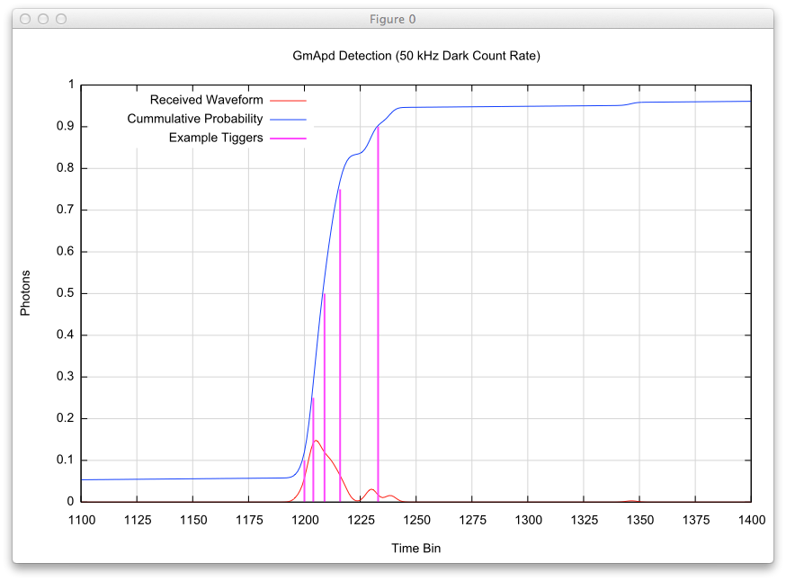
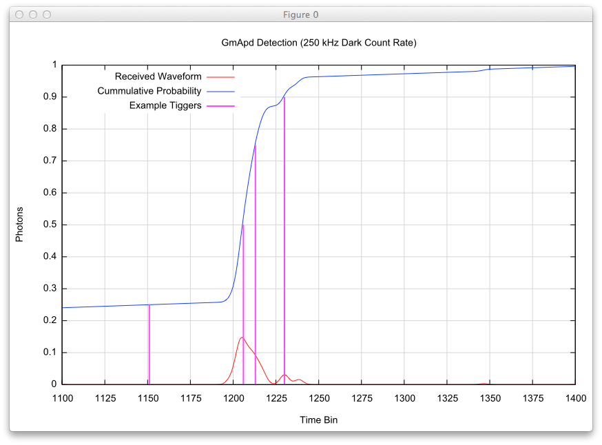
The current generation Geiger-mode devices can only trigger once while it is armed (during the listening window). Multiple returns with GmAPD system are obtained by imaging the same location multiple times. Because the detection is a Poisson process, a detector illuminated with the exact same waveform will not trigger at the same time on subsequent measurements. To illustrate this variations in trigger time, a low photon count waveform has been modeled with different dark count rates. Each plot shows where a single trigger would occur for different random values draw in the Monte-Carlo model of the detection.
The first simulation shows where 5 possible triggers would occur (for random values of 0.10, 0.25, 0.50, 0.75 and 0.90) with a DCR of 0.
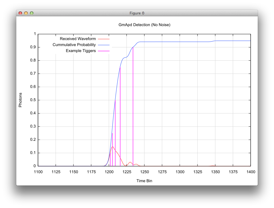
The second simulation employs the same random values, but with a DCR of 50 kHz. Note the bias in the cumulative probability in the lower time bins due to the increased noise. Even at this noise level, the location for these 5 possible triggers have not changed much compared to the previous no noise case.
The third simulation employs the same random values, but with a DCR of 250 kHz. Note the steeper slope in the cumulative probability in the lower time bins due to the increased noise. At this noise level, the random value of 0.10 has triggered outside (lower time bin) the plotted range and the triggers within the range have shifted to shorter time bins. Clearly the return near time bin #1150 would be considered a noise return since it does not correspond to any of the signal in the original waveform.
The GmAPD detector model is selected from the Detector Type menu on the Detector tab in the Lidar Detector Model. This provides the interface for the user to set the various parameters describing the detector’s characteristics.
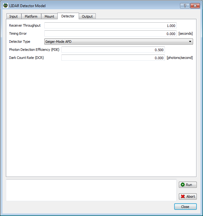
Photo-Multiplier Detection
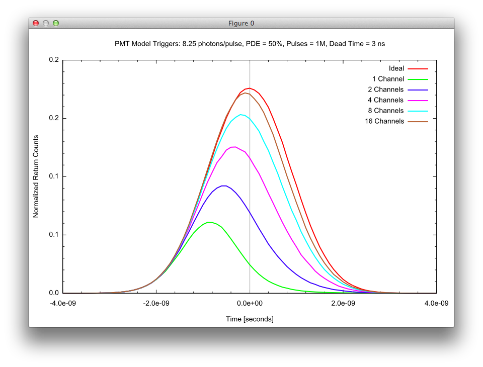
The photo-multiplier tube (PMT) model emulates the detection system employed in the ATLAS sensor that will be on the ICESat-2 satellite. The ATLAS receiver uses commercial photo-multiplier tubes that feature a 4x4 segmented anode. The ATLAS system has 2 sets of PMT devices, with one set receiving the "strong beam" spots and the other set receiving the "weak beam" spots. The "strong beam" PMTs route each of the 4x4 anodes to a separate discriminator, resulting in 16 channels. The "weak beam" PMTs have groups of 2x2 anodes summed and then routed to separate discriminators, resulting in 4 channels. Note that the grid of anodes do not provide an imaging capability. A complete description of the ATLAS system can be found in external documents written by the system architect Anthony J. Martino at NASA’s Goddard Space Flight Center (GSFC).
Because of the photon counting nature of this PMT-based detection architecture, the implementation of this detector model is very similar to that employed in the Geiger-Mode detection scheme described earlier. The PMT detector system is characterized using the same parameters employed by the Geiger-mode scheme, including the photon detection efficiency (PDE) and the dark count rate (DCR). The major additions to the Geiger-mode model found in this model are the following:
-
Multiple returns per channel including a "dead time" mechanism
-
Unlike the detectors and timers on the current generation Geiger-Mode systems, the PMTs and timers do not need to be "reset" after each trigger, which allows them to generate additional triggers for the same pulse. However, the detector timers have a "dead time" during which another trigger cannot be recorded. If an addition trigger is generated during the dead time, then the dead time window is restarted. If the received waveform has a large magnitude over a large number of time bins, then the detector can enter the dead time window and be constantly reset by additional triggers occurring within the dead time. This is referred to as a paralyzed state.
-
-
Multi-channel support to increase triggers and mitigate against "first photon" bias
-
The support for multiple channels arises from the segmented anode in the PMT device. This allows the output of each anode segment to be analyzed by a different timing circuit. The primary advantage of multiple channels is that multi-plexing the returned waveform into the channels divides the total flux among the anode segments (channels). As a result, strong returns are less likely to create "first photon" triggers that bias the range. In addition, the redundancy in channels means that the robustness of weak returns (where "first photon" bias is less of a concern) is also improved.
-
The probability of a trigger in a given time bin i can be computed using the following equation:
\( P(i) = \left [ 1 -\exp(-S(i) -w) \right ] \)
where S is the received active signal (in photoelectrons) and w is the noise rate per bin (photoelectron events per bin from passive background flux and dark count). When comparing this equation to the Geiger-mode detection equation presented earlier, the Geiger-mode equation has an explicit trigger exclusion term (driven by noise events) that extends all the way back to the start of the listening window. For this model, the "dead time" (which is a trigger exclusion mechanism) is part of the Monte-Carlo simulation (described below). The support for multiple channels is implemented by simply dividing the received waveform N times (16 times for the "strong beam" PMTs and 4 times for the "weak beam" PMTs) and repeating the detection process on the weighted waveform N times.
The modeling technique is as follows:
-
For each channel
-
For each time bin in the channel waveform
-
The probability of a trigger is computed for the current time bin using trigger probability equation.
-
A random number is pulled from a uniform distribution.
-
If the random value is less than the probability for the current bin, then the detector triggers.
-
If the trigger time is within the "dead time" of the previous trigger, then the last trigger time is updated but the trigger is not recorded.
-
If the trigger time is not within the "dead time" of the previous trigger, then the last trigger time is updated and the trigger is recorded.
-
-
-
This Monte-Carlo detection process is repeated until the there are no more bins left in the received waveform.
-
The impact of dead time is fewer overall detections since the device will miss trigger opportunities during dead time. The decrease in the number of detections can be observed when comparing the "Dead Time = 0 ns" to the other dead times in the plot below. In addition, the peak trigger time statistics will start to skew toward "first photon" events because later events will be blocked by the dead time. The plot below shows this effect by plotting the normalized number of returns per time bin for a 2 ns wide return pulse.
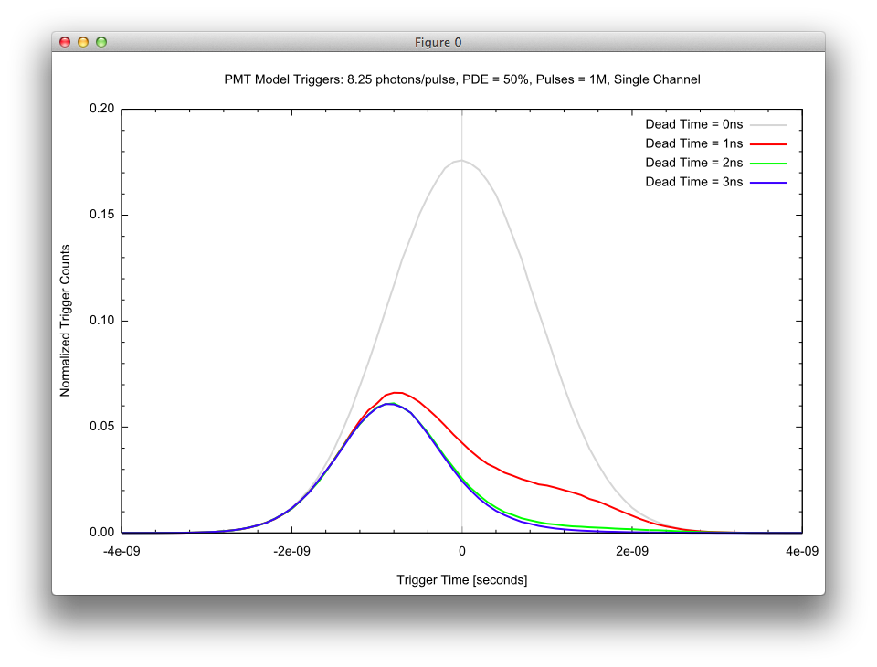
The impact of multiple-channels is to increase the total number of detections and to compensate for the "first photon" bias introduced by "dead time" in strong return scenarios. The plot below illustrates how more channels not only increases the total number of triggers (the area under the curve) but also how additional channels help to mitigate the "first photon" bias (the peak shifts back toward 0).
The PMT detector model is selected from the Detector Type menu on the Detector tab in the Lidar Detector Model. This provides the interface for the user to set the various parameters describing the detector’s characteristics.
Waveform Detection
One of the more interesting areas of development right now for laser radar are "waveform" LIDAR systems. Unlike Linear-mode (Lm) or Geiger-mode (Gm) system that collect a relatively small number of height measurements per GSD, a "waveform" LIDAR (wLIDAR) essentially digitizes the returned flux during the time window at some time resolution. That means you have intensity information at all the ranges rather than just a discrete set of them. This allows for some very complex post-processing of the data. Most wLIDAR systems feature a high performance, single-pixel detector coupled to a high performance digitizer. To obtain area coverage that detection system is coupled to a scanner that can provide across-track scanning while the airborne platform provides the along-track scanning via platform motion.
The BIN file created in "Stage 1" by DIRSIG contains for each pulse, the temporal flux for each pixel in the receiver array during the period that the array is armed (defined by a range gate or listening window) and is accompanied by a lot of meta-data including the precise absolute time of the current pulse, ephemeris like the platform location, platform orientation, platform relative pointing and information about the source and receiver. That portion of the data containing the temporal flux is basically what a wLIDAR system collects. The major difference is that the data produced by DIRSIG does not include an impulse response of the detector, A/D system, etc. Unlike the point clouds generated by conventional systems that can use the standardized LAS format, there has not yet been a widespread adoption of a file format for waveform LIDAR data. Note that the LAS 1.3 specification released in 2009 indeed has support for waveform data, but most operating sensors are still using home-grown data formats that were created before the recent LAS additions. For example, the data could be formatted into an ENVI image file employing the "spectral" dimension as a temporal dimension. Additional files can carry important meta data for the pulse including location of the area images, the source pulse profile, etc.
Is there any easy way to convert a DIRSIG BIN file into an ENVI image file so that the waveform can be visualized and processed? The answer is "Yes" and it doesn’t require conversion. The BIN file is a 3D cube of data with some metadata. The ENVI image header file can be used to directly import the BIN as long as:
-
The pulse data is not compressed using the lossless compression option
-
The file contains only a single pulse
The uncompressed data requirement is because ENVI cannot read the compressed data. Pulse compression can be turned off in the Output tab of the Receiver configuration. The single pulse requirement is because ENVI cannot handle skipping over the meta data between pulses in single, multi-pulse file. If you have a multi-pulse simulation, you can tell DIRSIG to generate a separate file for each pulse using the Generate files per capture option on the Output tab of the Receiver configuration.
The required ENVI header file can be created by hand using the following template:
ENVI
description = {DIRSIG .bin file}
samples = 128
lines   = 128
bands   = 302
header offset = 777
file type = ENVI Standard
data type = 5
interleave = bip
sensor type = Unknown
byte order = 0
wavelength units = Unknown
Here is an explanation of the various ENVI header file variables:
-
For this quick demo, a 128x128 array was model rather than scan a single pixel. Hence, the "samples" and "lines" are 128, respectively.
-
The listening window opened at 1.31e-05 seconds and closed at 1.34e-05 seconds, and had a time resolution of 1e-09 seconds. That results in 301 time bins "digitized". The file also includes the passive flux (Sun, Moon, etc.) as the first "band" in the cube. This results in 302 "bands" total.
-
The various meta-data headers in the .BIN file account for 777 bytes at the front of the file.
-
The spatial/temporal data is "band interleaved by pixel".
Product Generation
At this time the supplied Stage 2 processing tool provided with DIRSIG can output a 3D point cloud in either an ASCII/Text or a LAS 1.2 file. This 3D point cloud product may contains points generated by any noise mechanisms inherent to the detector model that generated the time-of-flight (ToF) measurement (a process that was discussed in detail in the last section for a variety of detection architectures).
|
|
In the LIDAR community, Level-0 (L0) data is usually associated with raw time-of-flight (ToF) measurements. Although these L0 time-of-flight values are internally computed by the respective detector models, there is not standard format for representing this data. Therefore, the DIRSIG Lidar Detector Model does not have the option to output L0 data at this time. |
|
|
In the LIDAR community, Level-1 (L1) data is usually associated with 3D point cloud data that has been generated by computing ranges from the L0 time-of-flight data and incorporating the platform location, platform orientation and platform-relative pointing. This L1 data is then passed onto higher level processing tools to perform tasks including filtering of noise points, flight to flight registration, etc. |
Incorporating Knowledge Errors
In order to go from Level0 time-of-flight data to Level-1 3D point clouds, each time-of-flight measurement must be converted to a range and then the platform location, platform orientation and platform-relative pointing must be used to locate that point in 3D space. The user can incorporate some common sources of "knowledge error" into this Level-0 to Level-1 processing.
|
|
"Knowledge’s errors" are errors that result from imperfect knowledge of some aspect of the data. Common sources of knowledge errors in LIDAR systems include uncertainty in the speed of light within air (due to spatial variations in temperature, relative humidity, etc.), and/or uncertainty in the platform location, platform orientation and platform-relative pointing. |
The Platform and Mount tabs allow the user to incorporate errors into the perfect knowledge of the platform location, platform orientation and platform-relative pointing that is provided via the BIN file. The user can selective specify temporally uncorrelated standard deviations about the true values for the six degrees of freedom for the platform ephemeris and the three degrees of freedom for the platform-relative pointing.
ASCII/Text Point Cloud Files
The options for the ASCII/Text output include:
-
Ability to write the points using either the native DIRSIG Scene ENU coordinates or a variety of geolocated coordinates.
-
The option to include a comment/header describing the multi-column file.
-
The option to include the task number for each point.
-
The option to include the pulse number for each point.
-
The option to include the pixel number for each point.
The ASCII/Text point cloud file writes a single line for each point
in the point cloud. Each line (record) contains columns that describe
the point. Depending on the detector model chosen and the options
selected, the number of columns and what each column is changes.
If the comment/header is included at the top of the file (the line begins
with #), it describes the column (fields) for each point record (each
line in the file). To clarify the format, a series of example files are
provided below.
LmAPD Detector with Scene/Local Coordinates Example
The following is an example ASCII/Text point cloud file under the following conditions:
-
The LmAPD Detector Model was chosen
-
The "Scene/Local" coordinate system was chosen
-
The "Include header" option was selected
# Generated by the DIRSIG Lidar Detector Model
# DIRSIG Release: 4.5.0 (r11943)
# Build Date: Feb 13 2013 09:50:58
# Detector Model: Basic LmAPD
#
# Column/Field Summary:
# Scene/Local Coordinate (X,Y,Z) [m], Return ID, Intensity
-27.8757 0.624295 -0.0887908 0 0.605323
...
3.8757 32.3757 -0.0887908 0 0.605323
|
|
The LmAPD detector model automatically adds the Return ID and Intensity fields as the last two fields in the record. If the user enables the Task ID, Pulse ID and/or Pixel ID fields, they appear before the Return ID and Intensity fields. |
The Return ID is a counter for each pixel that tags each return.
Within a pixel, the Return ID will start at 0 and increase for
each additional return found within that pixel.
The Intensity field is an indicator of the relative intensity
for the peak identified by the constant fraction discriminator (CFD).
LmAPD Detector with UTM Coordinates Example
The following is an example ASCII/Text point cloud file under the following conditions:
-
The LmAPD Detector Model was chosen
-
The "Universal Transverse Mercator (UTM)" coordinate system was chosen
-
The "Include header" option was selected
-
The "Include Task ID", "Include Pulse ID" and "Include Pixel ID" options were selected
# Generated by the DIRSIG Lidar Detector Model
# DIRSIG Release: 4.5.0 (r11943)
# Build Date: Feb 13 2013 09:50:58
# Detector Model: Basic LmAPD
#
# Column/Field Summary:
# UTM Location (zone, hemi, East, North, WGS84 Alt), Task ID, Pulse ID, Pixel X, Pixel Y, Pixel ID, Return ID, Intensity
17 N   707418.079  4777296.954      299.911 0 0 0 0 0 0 0.605
...
17 N   707448.852  4777329.659      299.911 0 0 0 0 0 0 0.605
|
|
The coordinate of the point is always the first N fields of the point record (line). A "Scene/Local" coordinate is 3 columns wide, a "Geodetic (Latitude/Longitude)" coordinate is 3 columns wide, a "Universal Transverse Mercator (UTM)" coordinate is 5 columns wide and an "Earth Centered, Earth Fixed (ECEF)" coordinate is 3 columns wide. |
The Task ID is a counter that starts at 0 and increases when the
points are generated from the next task. The Pulse ID starts at 0
and increases when the points are generated from the next pulse. The
Pixel ID option results in the X and Y coordinate of the pixel being
written, as well as the row-major
index of the pixel.
|
|
If any of these optional ID fields are not requested by the user (like in the previous example), they are simply omitted from the point records rather than included but assigned some sort of special/unused value. |
|
|
The Task ID field can be used to filter all the points generated during a given task in the simulation. |
|
|
The Pulse ID field can be used to filter all the points generated during a given pulse in the simulation. |
GmAPD Detector with Scene/Local Coordinates Example
The following is an example ASCII/Text point cloud file under the following conditions:
-
The GmAPD Detector Model was chosen
-
The "Scene/Local" coordinate system was chosen
-
The "Include header" option was selected
# Generated by the DIRSIG Lidar Detector Model
# DIRSIG Release: 4.5.0 (r11943)
# Build Date: Feb 13 2013 09:50:58
# Detector Model: Basic GmAPD
#
# Column/Field Summary:
# Scene/Local Coordinate (X,Y,Z) [m]
-27.8733 0.626674 0.210893
...
3.87333 32.3733 0.210893
|
|
The GmAPD model output does not automatically add any additional fields. If the user enables the Task ID, Pulse ID and/or Pixel ID fields, they appear after the point coordinate fields. |
A GmAPD detector is not capable of producing multiple returns per pixel or measuring intensity. Therefore, these fields are not automatically included in the output.
PMT Detector with Scene/Local Coordinates Example
The following is an example ASCII/Text point cloud file under the following conditions:
-
The PMT Detector Model was chosen
-
The "Scene/Local" coordinate system was chosen
-
The "Include header" option was selected
# Generated by the DIRSIG Lidar Detector Model
# DIRSIG Release: 4.5.0 (r11943)
# Build Date: Feb 13 2013 09:50:58
# Detector Model: PMT
#
# Column/Field Summary:
# Scene/Local Coordinate (X,Y,Z) [m], Channel ID, Return ID
-27.6231 0.626886 0.237637 0 0
...
3.87547 32.3755 -0.0594804 1 0
|
|
The PMT detector model automatically adds the Channel ID and Return ID fields as the last two fields of the record. If the user enables the Task ID, Pulse ID and/or Pixel ID fields, they appear before the Channel ID and Return ID fields. |
LAS Point Cloud Files
The LAS point cloud files contain the minimal headers and point meta-data descriptions described in the LAS 1.2 specification published by ASPRS.
Product Visualization
ASCII/Text Point Cloud Files
An ASCII/Text point cloud file has the flexibility of being imported into most 3D plotting and visualization tools. The following is a partial list of the tools commonly available for basic visualization of ASCII/Text files:
LAS Point Cloud Files
An LAS format point cloud file can be loaded into large number of commercial LIDAR exploitation packages. Many of these software packages offer free versions with limited analysis capabilities. However, these free versions usually support basic loading and visualization of LAS format files. The following is a partial list of the free tools available for basic visualization of LAS files:
Demonstrations and Examples
Single-Pulse
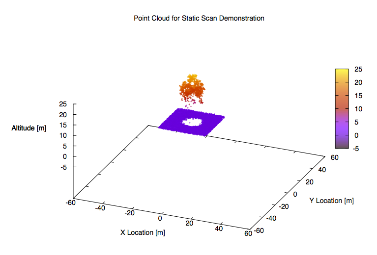
The LidarStatic1 demo shoots a single pulse onto a tree and receives that pulse onto a large format (128 x 128) array.
Multi-Pulse Scanning
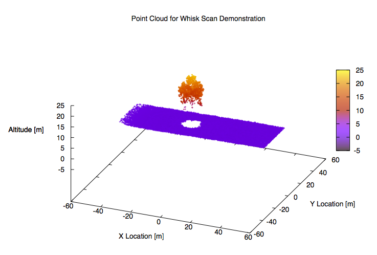
The LidarWhisk1 demo shoots a series of pulses while scanning in the across-track dimension.
Dynamic Range Gate
The LidarDynamicGate1 demo explains how the range gate can be adjusted on a pulse-by-pulse basis.
User-Defined Pulse
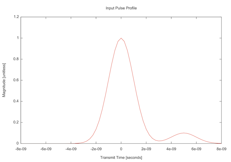
The LidarUserPulse1 demo explains how a user-defined temporal pulse profile can be incorporated into a simulation.
Jitter and Knowledge Errors
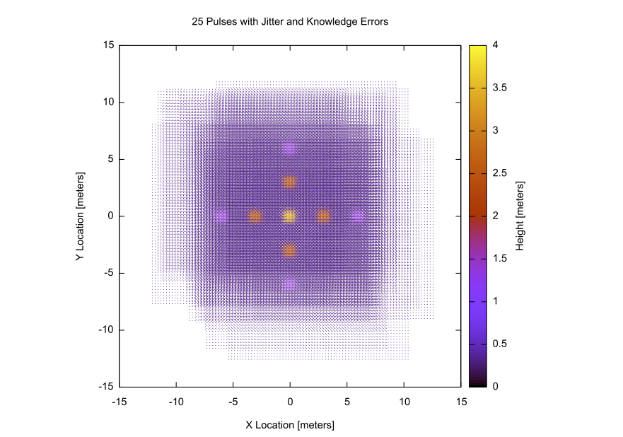
The LidarPointing1 demo demonstrates how command errors (jitter) and knowledge errors (GPS/INS noise) impact 3D point clouds.
Other Useful Information
Gaussian Width Conventions
Under the hood, the Gaussian form utilized in the DIRSIG model is based on the form normally used for the Normal Distribution:
\( f(x) = \frac{1}{\sigma \sqrt{2 \pi}} e^{-\frac{1}{2} \left ( \frac{x}{\sigma} \right )^2} \)
where \(\sigma\) is the standard deviation.
Beam Divergence Angle
The beam divergence angle (transverse width) of a Gaussian beam profile is supplied to DIRSIG as the half-angle at 1 sigma in the graphical user interface. The width of a Gaussian beam transverse profile can be measured at different intensity levels across the profile. Hardware descriptions can report this width parameter as the full-width at half maximum (FWHM), the half-width at 1/e, the full-width at 1/e, the half-width at 1/e2 or the full-width at 1/e2.
| Width | % of peak |
|---|---|
sigma |
60.6% |
FWHM |
50.0% |
1/e |
37.0% |
1/e2 |
13.5% |
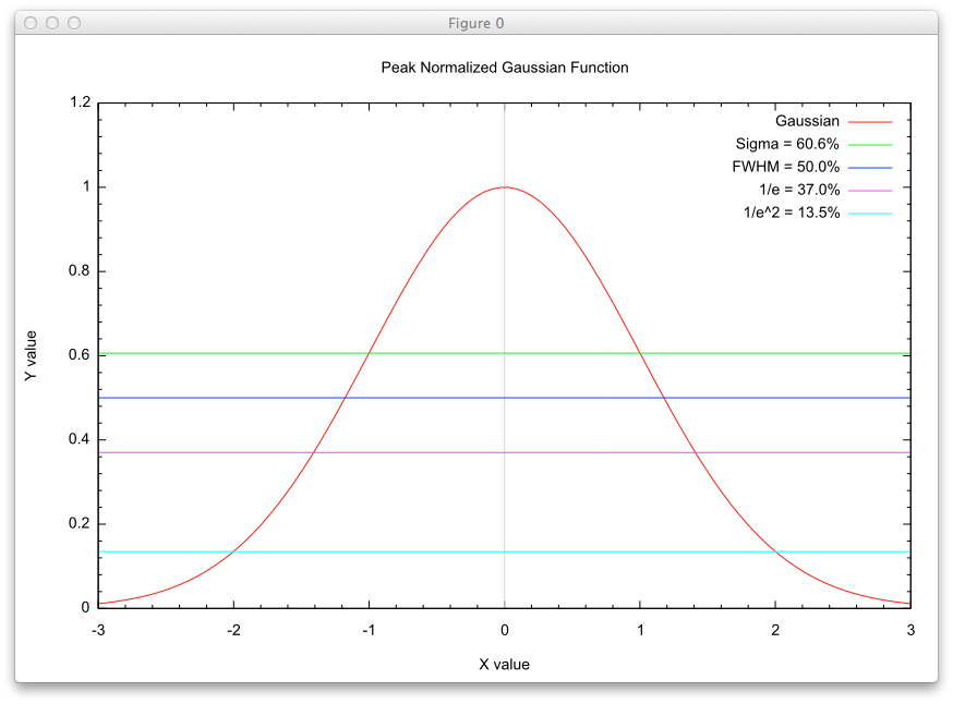
In order to convert these other values to the "half-angle is 1 sigma" convention employed in DIRSIG user interface, the following conversions are provided:
-
Half-angle is 1 sigma = 0.42466 full width at half maximum
-
Half-angle is 1 sigma = 0.70710 half width at 1/e
-
Half-angle is 1 sigma = 0.35355 full width at 1/e
-
Half-angle is 1 sigma = 0.50000 half width at 1/e2
-
Half-angle is 1 sigma = 0.25000 full width at 1/e2
|
|
If you hand-edit the .platform file, the widths in there are
stored as the full angle at 1 sigma.
|
Best Practices
The following recommendations are provided to help the user create robust simulations.
|
|
You will quickly find that most commercial systems do not have published specifications for important system specifications including the laser power (or pulse energy), the receiver spectral bandpass, etc. Many of these system parameters will need to be approximations, and some will have more impact on the resulting data than others. |
-
Verify the link budget (if possible)
-
The "link budget" (the number of laser photons expected to arrive at the receiver) is an extremely important operating characteristic of most LIDAR systems. If the link budget for a given system is known, you should always verify that your simulation matches after the first few pulses of the simulation have been completed. This can be accomplished using the command-line BIN File Analysis tool while a simulation is running.
-
"What are typical link budgets for common systems?"
-
We have never had a vendor give us a value for a commercial linear-mode system. However, we suspect that they run at 10-100 photons/pixel/pulse.
-
Geiger-mode and other photon counting systems should have an average value of 0.1 - 2.0 photons/pixel/pulse, depending on the photon detection efficiency of the detector.
-
-
-
Verify the point density (if possible)
-
Although most commercial systems will not tell you important engineering specifications, they usually report important product specifications including the point density, or the number of points per area. For example, most commercial airborne systems will provide 10-20 points/meter2.
-
After the first few pulses have been generated, an initial point cloud can be generated. The DIRSIG tools do not have a way to calculate the point density for you, but most of the commercial tools described in the Product Visualization section can perform this calculation.
-
Check if the point density is symmetric
-
Is the point density uniform (symmetric in the along- and across- track directions) or denser in one direction?
-
Is this expected? If not you then might need to change the pulse rate, scan rate and/or platform velocity.
-
-
-
Be careful about the receiver channel response width
-
The relative spectral response (RSR) of the receiver (especially the spectral width) is critical for daylight simulations. A wider RSR will allow more background (reflected solar or lunar) light to arrive at the detector. Since this background flux arrives constantly, it carries no range information and can lead to noise.
-
-
Be careful about the channel response and bandpass configuration
-
This advice applies to channel response configurations across all the modalities in DIRSIG. If your channel has a relative spectral response that is 8 nm wide and centered on 1064 nm, then your spectral bandpass should range from 1060 - 1068. Making the bandpass wider will only increase the run-time (slightly) and making it narrower will truncate the magnitude of the captured signal.
-
-
Verify the beam spot size vs. receiver FOV (if possible)
-
Some systems have the laser transmitter underfill the receiver FOV (the projected spot of the laser is entirely contained with in the FOV) to maximize the number of photons received at the receiver. Other systems overfill the receiver FOV (the projected spot of the laser is larger than in the FOV) in order to have more uniform illumination within the FOV (because most beam spots are peaked in the center and trail off at the sides).
-
Although key parameters like the beam divergence angle or the pixel IFOV may not be available, sometimes the transmitter vs. receiver "optical coupling" or similar parameter is provided that attempts to characterize the relative solid angle of the beam and receiver. If available, always check this value with some simple geometry calculations.
-
-
Always use pixel sub-sampling
-
The use of pixel sub-sampling is important for the LIDAR modality. Recall that the detector samples the scene with rays that have zero area. If a single sample ray is used for each detector element (pixel) then a single object will be found at a given range. Although multiple bounce photons may contribute so additional information at other times of flight, the received waveform will be dominated by flux from this single object. The only way to capture contributions from multiple objects that are present at other ranges within the pixel IFOV is to spatially sample the pixel.
-
"How much sampling?" is a difficult question to answer because it is driven by the geometric complexity of the scene and the ground sampling distance (GSD) of the receiver element. The following examples are provided to help the user consider their specific scenario:
-
Always prefer odd size sampling grids so that a sample ray can collect information for the center of the pixel.
-
For a large area, bare terrain simulation you can probably get away with 3x3 sampling regardless of the GSD because there is only a single object within each IFOV and the variation within that IFOV is not expected to be high.
-
For some of our waveform LIDAR simulations of tree canopies that used high resolution tree geometry models (with species specific shaped leaves), we used 7x7 samples grid to make sure we captured the range diversity of leaves within a pixel IFOV.
-
For some of our ICESat-2 simulations where we had a 12.5 meter ground spot and ice sheet geometry with 1 meter spatial resolution we used a 15x15 sample grid for each pixel.
-
-
-
Prefer the Direct+PM radiometry method
-
This provides the fastest run-times and the most robust radiometry result.
-
This is selected using the Use photon mapping for higher returns only option in Options Editor (or the
.optionsfile).
-
-
Carefully setup the photon mapping parameters
-
The Direct+PM radiometry approach requires the user to configure the photon mapping setup, which is contained in the Options Editor (or the
.optionsfile). The user must define the following three parameters:-
The Maximum source bundles, which defines the number of photon bundles (packets) that can be shot from the source.
-
The Maximum bounces per bundle, which defines the number of reflections that are followed before a bundle will terminate.
-
The Maximum events in map, which defines the maximum number of reflection, absorption, scattering, etc. events that will be stored in the photon map.
-
-
The Maximum bounces per bundle variable is used to make sure that the multiple bounce calculations have an exit condition even if your scene is a "house of mirrors" (highly reflective such that photon bundles are rarely absorbed). In real-world scenes with modest reflectances (10-40%), then the default value of
4is usually fine. If you are modeling a high albedo scenario (snow, ice, clouds) then a larger number should be considered. -
The Maximum events in map variable is configured to make sure the a event density within the photon map is sufficient to compute robust multi-bounce impacts. The recommendations we put forth here are application specific:
-
A photon counting system typically samples the same locations multiple times in order to have enough data to remove the noise added by the detector. Therefore, a good rule of thumb is to have 10-100 events for each pixel in the receiver. For a 32x32 GmAPD array (with 1,024 pixels) that would be 10,000 to 100,000 events.
-
A linear-mode system typically has a higher link budget and is less sensitive (potentially) to multi-bounce returns. Therefore, a a good rule of thumb is to have 100-1000 events for each pixel in the receiver. Since most linear mode systems have only a single detector (pixel), then that would be 1,000 to 10,000 events.
-
-
The Maximum source bundles variable should always be greater than or equal to the Maximum events in map variable
-
This is because each source bundle generates a minimum of 1 event per bundle (if every bundle is immediately absorbed) and more than 1 even per bundle if each bundle is reflected or scattered at least once.
-
-