The BasicPlatform plugin was created to provide backward compatibility in DIRSIG5 for the sensor collection capabilities in DIRSIG4.
The inputs to this plugin are the DIRSIG4 era platform, motion (either a GenericMotion or a FlexMotion description) and a tasks file. This allows the plugin to emulate the sensor collection capabilities in DIRSIG4. For more details, see the usage section at the end of this manual.
Related Documents
-
Platform Motion
-
Instruments
Implementation Details
Spatial and Temporal Sampling
This sensor plugin performs spatial and temporal sampling differently than DIRSIG4 did. Specifically, DIRSIG4 used discrete sampling approaches to separately sample the spatial and temporal dimensions of flux onto a given pixel and DIRSIG5 simultaneously samples the spatial and temporal dimensions with uniformly distributed samples.
In DIRSIG4, the amount of sub-pixel sampling was controlled on a per focal plane basis using rigid N x M sub-pixel sampling. Furthermore, delta sampling vs. adaptive sampling was a choice for the user. In contrast the BasicPlatform plugin uniformly samples the detector area and the number of samples used for each pixel is adaptive and driven by the convergence parameters. In general, the entire spatial response description in the input file is ignored by this plugin.
The DIRSIG4 temporal integration feature included an integration time and an integer number of samples to use across that time window. The temporal sampling approach brute-force resampled the entire detector for each sample, which resulted in a proportional increase in run-time. The DIRSIG5 BasicPlatform plugin ignores the number of temporal samples and instead uniformly distributes the ray times across the integration time window.
Instrument Types
Basic Instrument
Lidar Instrument
This instrument is used when a mono-, bi- or multi-static LIDAR instrument is being modeled. It generally extends the BasicInstrument capability by adding the capture of time-of-flight data via the lidar capture method.
Data Recorder Instrument
This instrument is used to collect platform or mount relative location and orientation telemetry during a simulation. It can be used to emulate the collection of global position system (GPS) and/or inertial measurement unit (IMU) data.
Capture Methods
DIRSIG4 and this plugin in DIRSIG5 feature different capture methods, which defines what happens to the at-aperture radiance during collection. There are three widely used methods, with the first two reserved for passive electro-optical (EO) and infrared (IR) collection scenarios and the third for active EO/IR (aka, lidar) collection scenarios.
Simple Capture Method
This is the most commonly used method. This method allows the user to define how the incident radiance is spectrally, spatially and temporally integrated. It provides support for basic apetures, spectral response functions and the ability to convert the incident radiance to digital counts (DCs) through a internal detection model.
Raw Capture Method
This mode is typically used when the user plans on using their own external detection model. The output of this method is a spatially and spectrally "oversampled" (more samples than the ultimate output) data cube. A spatially oversampled incident radiance field provides an external optics and detection model with sub-pixel samples in order to perform modulation transfer function (MTF) calculations and resample to the final sensor resolution. The spectrally oversampled dimension provides enough resolution for spectral integration into channels that might vary across the focal plane.
Lidar Capture Method
This capture method is used with laser radar receivers, and adds to the general feature set of the "simple" capture method the ability to output the incident flux as a function of time. Unlike the previously discussed passive capture methods that output an ENVI image file, this capture method outputs spatial x spatial x time data cubes using the DIRSIG BIN format.
Output Units
The internal radiometric units of the DIRSIG5 radiometry core are:
\begin{equation} \frac{\mathrm{watts}}{cm^2 sr \mu m} \end{equation}
The final output units can differ, depending on the output capture method and the respective options set for that capture method. This section focuses on the output units for data generated using the simple and raw capture methods, which store the output into ENVI image files. The output units of the lidar capture method in the BIN file is always photons.
|
|
The ENVI Image Header will always include
the data units variable that specifies the units of the image data.
|
At Aperture Units
By default, the BasicPlatform plugin using the Simple capture method produces an at aperture radiometric data product that is by default in spectrally integrated radiance units of watts/(cm2 sr).
Depending on the various options set, the units produced by the Simple capture method can change. For example:
-
The flux term can be switched from watts to milliwatts, microwatts, photons/second or electrons/second by manipulating the
fluxunitsattribute to in the<imagefile>element. The options are:-
watts(default) -
milliwatts -
microwatts -
photonspersecond -
electronspersecond(assumes response is quantum efficiency)
-
-
The area term can be switched from per cm2 to per m2 by manipulating the
areaunitsattribute in the<imagefile>element. The options are:-
cm2(centimeters2, default) -
m2(meters2)
-
<imagefile> element with attributes for a <focalplane>. <imagefile areaunits="cm2" fluxunits="watts">
<basename>circle_psf</basename>
<extension>img</extension>
<schedule>simulation</schedule>
<datatype>5</datatype>
</imagefile>The flux and area units can also be maniupulated in the Output Files tab of the Simple Capture Editor dialog in the graphical user interface.
At Focal Plane Units
If an aperture is defined, the resulting acceptance angle of the aperture is incorporated and the radiance at the aperture (watts/(cm2 sr)) is converted to an irradiance at the focal plane (watts/cm2). This acceptance angle is defined via the G# (see Schott), which is a function of the focal length, aperture diameter and aperture throughput (geometric and optical).
The options for aperture are defined in the <properties>
element of the <instrument> and in the Advanced tab of the
Instrument Editor:
<properties> element for an <instrument>. <properties>
<aperturediameter>0.09</aperturediameter>
<aperturethroughput>1</aperturethroughput>
<focallength>1140</focallength>
</properties>The F# of the system is then defined as:
\begin{equation} F\# = \frac{L_f}{D_A} \end{equation}
where Lf is the focal length and DA is the aperture diameter. The G# is then defined as:
\begin{equation} G\# = \frac{1 + (4 \cdot F\#^2)}{\tau_A \pi} \end{equation}
with units of per steradian (1/sr).
The at focal plane irradiance (E) can then be computed from the at aperture radiance (L) as:
\begin{equation} E = \frac{L}{G\#} \end{equation}
A change in quantity from radiance to irradiance results in a change of units as well as the per steradian term has been removed:
-
Flux/(Area sr) → Flux/Area
For example, an at aperture radiance in watts/(cm2 sr) will now be a at focal plane irradiance in watts/cm2.
With Temporal Integration
Enabling "temporal integration" will integrate the seconds in the flux term resulting in (depending on the flux term settings):
-
Watts → Joules
-
Milliwatts → Millijoules
-
Microwatts → Microjoules
-
Photons/second → Photons
-
Electrons/second → Electrons
The options for temporal integration are defined in the <capturemethod>
element of a <focalplane> and in the Clock tab of the Focal Plane
Editor:
<capturemethod>. <temporalintegration>
<time>0.1</time>
</temporalintegration>With Channel Normalization
It is not uncommon for spectrometers to output units in spectral radiance since the data is usually treated as a spectrum. In this case, the signal onto the detectors is spectrally integrated by the individual channel but the data delivered to users is calibrated and normalized by the integral of the channel.
\begin{equation} L_C = \frac{\int L_i(\lambda) R_C(\lambda) d\lambda}{\int R_C(\lambda) d\lambda} \end{equation}
where LC is the spectral radiance for a channel, Li is the incident spectral radiance and RC is the spectral response of the channel at the wavelength. Hence, the spectral integration (numerator) removes the per wavelength units but the normalization (denominator) adds it back in.
With the Detection Model
If the internal detector model is configured, the output units are simply in digital counts (DCs).
Summary
To assist in understand the interaction of the various units options, the following table is provided with a subset of possible combinations:
| Flux Units | Area Units | Aperture Defined | Temporal Integration | Channel Normalization | Final |
|---|---|---|---|---|---|
Watts |
cm2 |
No |
No |
No |
Watts/(cm2 sr) |
Watts |
cm2 |
No |
No |
Yes |
Watts/(cm2 sr um) |
Watts |
cm2 |
Yes |
No |
No |
Watts/cm2 |
Watts |
cm2 |
Yes |
No |
Yes |
Watts/(cm2 um) |
Watts |
cm2 |
No |
Yes |
No |
Joules/(cm2 sr) |
Watts |
cm2 |
Yes |
Yes |
No |
Joules/cm2 |
Photons/sec |
cm2 |
No |
No |
No |
Photons/s/(cm2 sr) |
Photons/sec |
cm2 |
Yes |
No |
No |
Photons/s/cm2 |
Photons/sec |
cm2 |
No |
Yes |
No |
Photons/(cm2 sr) |
Photons/sec |
cm2 |
Yes |
Yes |
No |
Photons/cm2 |
Standard Features
Truth Collection
The parameters gather by the various truth collectors are stored into a 3-D image cube, where each "band" in the image contains information about a specific image formation parameter.
|
|
For specifics on the format of these binary image files, consult the Output Image Format document. |
The truth collectors can be configured in the user interface, or manually
within the .platform file. Similar to the options for output image files
produced by the focal plane capture methods, the user can specify the output
file "schedule", which allows for:
-
A single image file for the whole simulation,
-
A separate image file for each task, or
-
A seperate image file for each capture
The XML schema for the truth collection in the .platform file is as
follows:
          <focalplane>
            ...
            <truthcollection>
              <enabled>true</enabled>
              <imagefile>
                <basename>example_truth</basename>
                <extension>img</extension>
                <schedule>simulation</schedule>
              </imagefile>
              <collectorlist>
                <collector>
                  <name>Material</name>
                </collector>
                ...
              </collectorlist>
            <truthcollection>
          </focalplane>
where each focal plane can have one or more <truthcollection>
elements configured. The <collectorlist> element contains one or
more <collector> elements that configure truth collectors by
providing either an individual collector name (e.g., materialindex)
or the name of a truth set (e.g., material).
It should be noted that some truth collectors include additional variables. For example, the abundance collector takes either a material ID (label) or a geometry tag.
In the material abundance mode, the <materials> element is provided and
contains a comma separated list of material IDs for target materials for
which sub-pixel abundances will be collected:
                <collector>
                  <name>Abundance</name>
                  <materials>10,grass</materials>
                </collector>
In the tagged geometry abundance mode, the <tags> element is provided
and contains a comma separated list of tags for target geometries for
which sub-pixel abundances will be collected:
                <collector>
                  <name>Abundance</name>
                  <tags>truck,car</tags>
</collector>|
|
Multiple truth <truthcollection> elements can be described with
each collecting different truth types and routing them to separate
files. In addition to funneling specific data to specific files,
this also allows groups of collectors to be easily enabled and
disabled.
|
Advanced Features
This plugin includes a few advanced features that should become permanent features at some point in the future.
|
|
These advanced feature configurations are not supported by the
graphical user interface (GUI) and will get deleted if the user loads
and saves the .platform file in the Platform Editor.
|
Hypersampling
The DIRSIG5 radiance convergence algorithm powers the adaptive sampling approach to the simulation solution. It allows pixels that are less complex spatially, spectrally or temporally to use fewer samples (paths), and conversely more complex pixels to use more samples (paths). The algorithm initializes itself with an estimate of the pixel radiance using a minimum number of paths (Nmin). It then incrementally adds more paths to the radiance solution and compares the radiance at the reference wavelength from the previous N-1 sample solution to the current N sample solution. If the radiance difference is greater than the threshold, then another sample is added to the solution until the threshold is satisfied or the maximum number of samples (Nmax) is reached.
One of the failure corner cases for this algorithm is when there is a significant sub-pixel contribution that is missed by the minimum number of samples. For example, a small object within a pixel that is a major contribution to the pixel due to it having a high reflectance or a high temperature. If the object is small (in terms of area), it could easily be missed by a low number of minimum samples (Nmin). Hence, the solution could converge after only Nmin samples with all the samples having randomly sampled the portion of the pixel represented by something other than this small but important object. This corner case can also manifest with larger targets that contain a small but significant component. For example, a small chrome feature on a car that reflects a solar glint in the reflective region or a hot exhaust pipe in the thermal region. Increasing the minimum number of samples would increase the likelihood that such small but important contributors are not missed, but increasing the minimum number of samples for all the pixels can have a dramatic impact of run-time.
Ideally, we want a way to automatically identify specific pixels that contain these corner cases and utilize more samples in those pixels only. Although it is not automatic, this can be accomplished by using the hypersampling feature that allows the simulation to dynamically increase the Nmin and Nmax samples used in the convergence algorithm for select pixels. To utilize the feature, the user needs to label important targets and specify a sampling multiplier that increases the sample rates when any of the labeled targets are within a pixel. When a pixel IFOV overlaps these labeled targets, the Nmin and Nmax values will be increased by a user-defined multiplier.
Labeling Important Objects
The key step is to label instances that are "important". Instance
labeling is only supported in the GLIST file and is accomplished by
setting the name (or tags) attribute in either a static or dynamic
instance to start with the specific string "::IMPORTANT::".
</geometrylist>
  ...
  <object>
    <basegeometry>
      <obj><filename>objects/example.obj</filename></obj>
    </basegeometry>
    <staticinstance name="::IMPORTANT::">
      ...
    </staticinstance>
    ...
  </object>
</geometrylist>
Instances of any type of base geometry (GDB, OBJ, GLIST or primitive) can be flagged as important. Not all instances of a given base geometry need to be labeled. For example, in some cases you might only want to label "fast moving" instances as important.
|
|
If the ::IMPORTANT:: string is added to the
tags for the <object>, all the instances
will inherit that tag and will get hyper-sampled.
|
Enabling Hypersampling
To enable hypersampling in sensor, the user must set the Hypersampling multiplier, which can be done in the GUI:
-
❏ Open the Focal Plane Editor for the desired focal plane.
-
❏ Select the Response tab and click the Edit button.
-
❏ In the Simple Capture Editor, select the Spatial Response tab.
-
❏ Set the Hypersampling multiplier variable to a value greater than
1.
This can also be configured by directly editing .platform file and
setting the appropriate element. The hypersamplingmultiplier
element specifies a multiplier that modifies the minimum and maximum
number of samples used in each pixel when an important target
overlaps the pixel IFOV. The use of this special element is shown
within the <samplestrategy> element in the example below:
          <focalplane enabled="true" name="Example FPA">
            <capturemethod type="simple" name="Simple">
              <samplestrategy type="central">
                <hypersamplingmultiplier>50000</hypersamplingmultiplier>
              </samplestrategy>
              <imagefile>
                ...
              </imagefile>
              <spectralresponse>
                ...
              </spectralresponse>
              <spatialresponse>
                ...
              </spatialresponse>
            </capturemethod>
            ...
          </focalplane>
See the SubPixelObject1 demo for a working example.
Lens Distortion
The ideal pinhole camera approximation employed by this plugin can be enhanced via the use of the built-in lens distortion model. This common 5-parameter distortion model allows the user to introduce common distortions including barrel and pin cushion. The governing equation has 3 radial terms (k1, k2 and k3) and 2 tangential terms (p1 and p2) that define the transform of an undistorted point (x,y) on the focal plane into a distorted point (x',y').
\begin{eqnarray} x' &=& x \cdot (1 + k_1 r^2 + k_2 r^4 + k_3 r^6) + 2p_1 xy + p_2(r^2 + 2x^2)\\ y' &=& y \cdot (1 + k_1 r^2 + k_2 r^4 + k_3 r^6) + 2p_2 xy + p_1(r^2 + 2y^2) \end{eqnarray}
Units for x and y are in focal lengths and centered about the principal point of the instrument.
Since DIRSIG is a reverse ray-tracing approach, the plugin is performing the inverse of this mapping to compute the appropriate rays to sample the correct regions of the object plane. It should be noted that these equations are not invertable, so the inversion is performed using an iterative solution to find the undistorted point (x,y) from a distorted point (x',y') on the focal plane.
The 5-parameter model can be configured via the GUI:
-
❏ Open the Instrument Editor for the desired instrument.
-
❏ Select the Advanced tab.
-
❏ Select the Five Parameter Model (DIRSIG5 only) from the dropdown menu.
-
❏ Set the five parameter coefficients.
The distortion model can also be configured via the <distortion>
element insider the <properties> of a given instrument.
<instrument type="generic" name="Name">
<properties>
<focallength>35</focallength>
<distortion>
<k1>5</k1>
<k2>2.5</k2>
<k3>-100</k3>
<p1>0.1</p1>
<p2>0.05</p2>
</distortion>
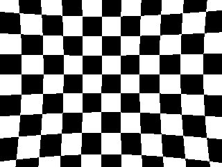
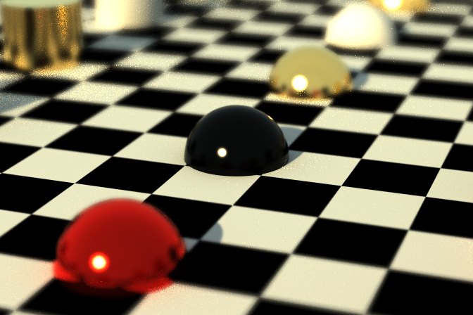
</properties>The parameter set above produces a pronounced "pincushion" distortion when looking at a checkerboard pattern.
See the LensDistortion1 demo for a working example.
Rolling Shutter
A "capture" of 2D imaging array has two distict phases: (1) integration energy indicent onto the detectors and (2) the readout of the electrons from those pixels. The readout rate (or frame rate) is the inverse of the total time for the array to both integrate and readout the pixels and reflects how often a new frame of data can be acquired. In general, increasing the integration time (how long pixels "soak up" photons) is independent of the read out time (how long it takes to read how many photo-electrons were generated in the pixels).
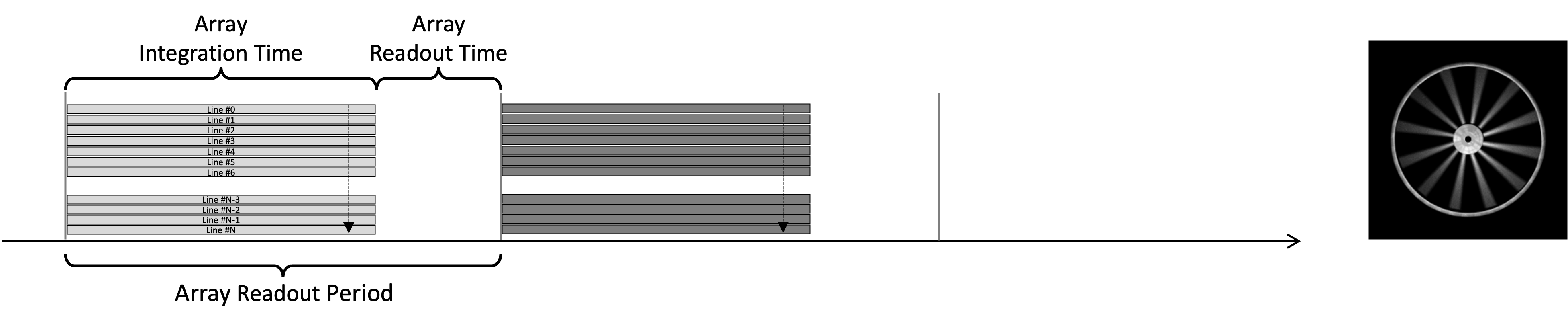
A global shutter array will synchronously integrate all the pixels at the same time and then read out all the pixels before starting the cycle over for the next capture. While the pixels are being read out, they cannot be integrating. Reading out a row of pixels can be thought of as (generally) a constant time operation. Consider a 100 line array that takes 0.0001 seconds to read out each line. Therefore, it takes 100 lines x 0.0001 seconds/line = 0.01 seconds to read out all the lines. If we let all the pixels integrate for 0.04 seconds, then that means a single integration and readout period would be 0.04 + 0.01 = 0.05 seconds. This yields an effective readout rate (or frame rate) of 1 / 0.05 seconds = 20 Hz. In a global shutter, all the pixels integrate at the same time but the integration time is fraction of the total readout period.
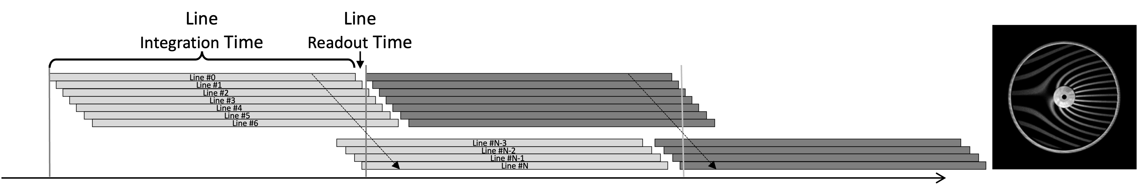
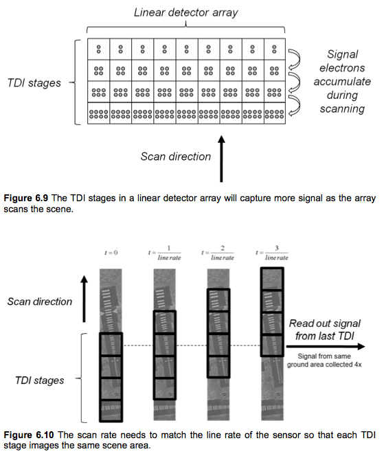
A rolling shutter array will asynchronously and independently integrate and read out lines of pixels. Doing so means that while one line of pixels is being read out, other lines can continue to integrate. For a given frame rate, this allows the integration time to increase. To see why, consider working backward from the previous scenario used for the global array scenario. At 20 Hz, we have to read out all the lines every 0.05 seconds. If we only have to read out a single line every 0.05 seconds, then the integration time for that line could be 0.05 - 0.0001 = 0.0499 seconds. This is significantly higher (almost 20% longer) than the 0.0400 seconds for the global shutter case. But we still need to integrate and read out all the lines, so to accomplish this we asynchronously integrate and read out lines. At time = 0 seconds we start to integrate the first line. After 0.0001 seconds, we start to integrate the next line, and 0.0001 seconds later we start to integrate the next line, etc. When the first line is done integrating after 0.0499 seconds, we read it out which takes 0.0001 seconds. That line can start integrating again as we move on to read out the next line which had its integration start delayed by 0.0001 seconds. The process repeats where as we finish reading out one line, the next line is ready to be read out, and this line-by-line read out rolls through the array. Effectively, the frame rate is still 20 Hz because every 0.05 seconds we read out the first line, but the lines are no longer being integrated at the same time. The advantange is that the effective integration time is greater (20% in this example). However, because lines are not integrating at the same time, artifacts can appear in objects in motion like the "shredding" of the spinning wagon wheel in the example below.
A couple of useful tips and checks:
-
The term "lines" and "rows" are sometimes used interchangably in this context.
-
Since the line "readout time" is used to delay when the integration of the next line starts, this term is sometimes referred to as the line "delay time".
-
The readout time is usually dependent on the number of pixels. Therefore, more pixels generally leads to longer readout times.
-
The readout time is usually independent of the integration time for the pixels. Therefore, a longer integration time usually does not impact the readout time.
-
At the limit (where the integration time is 0), the number of lines in the array multiplied by the line read out time must be less than the frame read out period, which is the inverse of the readout or frame rate.
Exponential Temporal Decay Response
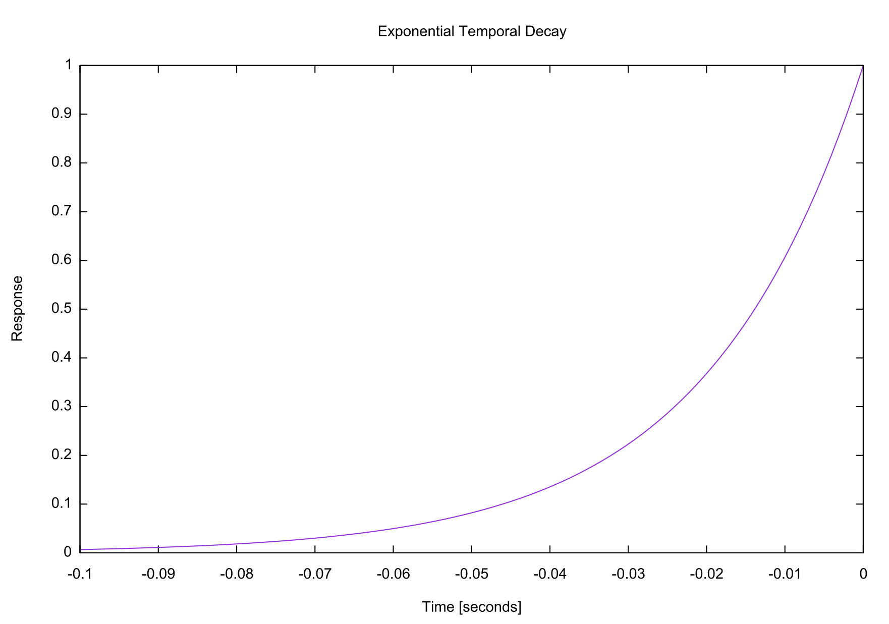
A traditional integration response, accumulates signal onto the detector over a finite time window, with an equal response as a function of time within that window. The optional temporal decay response reflects the behavior common in a microbolometer type array, where the array is still read out at a constant rate, but the signal is proportional to the signal received over a longer time period and with an exponential weighting.
\begin{equation} w = \exp^\frac{1}{\mathrm{decay~time}} \end{equation}
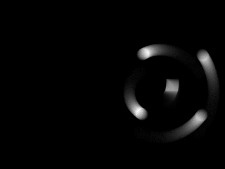
For example, when modeling a 20 ms decay time, the signal is accumulated over a nearly 100 ms time window, but is exponentially biased toward then end of that time window (see below):
This type of temporal response typically produces "streaking" effects with moving objects in the scene or when the camera makes quick movements. The image example below features a set of of 4 spheres rotating around a box. The fading tails behind the rotating spheres reflect the decaying response to where the spheres have been when the array is read out.
This feature can be configured via the graphical Platform Editor or
directly within the raw or simple capture method in the .platform file:
              <temporalintegration tdi="false">
                <time>0.01</time>
                <samples>10</samples>
</temporalintegration> <temporalintegration tdi="false">
<decay>0.02</decay>
<samples>10</samples>
</temporalintegration>|
|
As a reminder, the <samples> are ignored by the DIRSIG5
BasicPlatform plugin, which randomly distributes temporal
samples as part of the simultaneous spatial (angular) and
temporal Monte-Carlo sampling process.
|
Time-Delayed Integration (TDI)
Time-delayed integration (TDI) is a strategy to increase signal-to-noise ratio (SNR) by effectively increasing the integration time for each pixel. Rather than using a single pixel with a long integration time, TDI uses a set of pixels with a short integration time that will image the same location over a period of time. This is usually utilized in a pushbroom collection system, where a 1D array is scanned across a scene using platform motion to construct the 2nd dimension of the image. TDI is typically accomplished by using a 2D array in pushbroom mode and using the 2nd dimension of that 2D array as TDI "stages" that will be used to re-image the same location as the system as the array is scanned by the platform in the along-track dimension. The figure below illustrates this concept [1].
In order to use the TDI feature, you need to have the following
components setup in the <focalplane> configuration in the
.platform file:
-
The Y dimension of the detector array is assumed to be the TDI stages. Hence, the
<yelementcount>in the<detectorarray>should be set to indicate the number of stages desired (greater than 1). -
The temporal integration time needs to be set. Hence, the
<time>element in the<temporalintegration>should be set to a non-zero length. -
The TDI feature needs to be explicitly enabled. This is accomplished by setting the
tdiattribute in the<temporalintegration>element to "true". -
To introduce detector noise, you need to enable and configure the built-in internal detector model.
Below is an example excerpt from a .platform file that has these
components configured. In this case, the array has 12 stages of TDI
(see the <yelementcount> element.
          <focalplane>
            <capturemethod>
              ...
              <temporalintegration tdi="true">
                <time>2.0e-05</time>
                <samples>1</samples>
              </temporalintegration>
              <detectormodel>
                <quantumefficiency>1.0</quantumefficiency>
                <readnoise>20</readnoise>
                <darkcurrentdensity>8.0e-07</darkcurrentdensity>
                <minelectrons>0</minelectrons>
                <maxelectrons>10e+02</maxelectrons>
                <bitdepth>12</bitdepth>
              </detectormodel>
              ...
            </capturemethod>
            <detectorarray spatialunits="microns">
              <clock type="independent" temporalunits="hertz">
                <rate>50000</rate>
                <offset>0</offset>
              </clock>
              <xelementcount>250</xelementcount>
              <yelementcount>12</yelementcount>
              <xelementsize>2.00000</xelementsize>
              <yelementsize>2.00000</yelementsize>
              <xelementspacing>2.00000</xelementspacing>
              <yelementspacing>2.00000</yelementspacing>
              <xarrayoffset>0.000000</xarrayoffset>
              <yarrayoffset>0.000000</yarrayoffset>
              <xflipaxis>0</xflipaxis>
              <yflipaxis>0</yflipaxis>
            </detectorarray>
          </focalplane>
See the TimeDelayedIntegration1 demo for a working example.
|
|
Although the stages are spatially and temporally sampled separately, the stages are solved as a single "problem" in the DIRSIG5 radiometry core. That means the paths per pixel is distributed across all the stages. Therefore, we recommend that you proportionally increase the convergence parameters as you increase the number of stages. For example, if you have N stages, you might consider increasing the minimum and maximum number of paths/pixel by N. |
Color Filter Array (CFA) Patterns
|
|
This feature requires manual editing of the .platform file
because the graphical user interface does not support it.
The feature configuration will be lost of you open and save the
.platform file from the Platform Editor.
|
As an alternative to assigning a focal plane one (or more) channels that
are modeled at every pixel, the option also exists to generate mosaiced
output of a color filter array (CFA) that can be demosaiced as a post
processing step. The currently supported CFA patterns include the Bayer
and TrueSense patterns. These are configured by adding the
<channelpattern> section to the <spectralresponse> for a given
focal plane. Each channel pattern has a list of pre-defined "filters" that
must be mapped to the names of channels defined in the <channellist>.
Examples for each pattern are shown in the following sections.
|
|
The DIRSIG package does not come with a tool to demosaic images
produced with CFA patterns.
Standard algorithms
are available in a variety of software packages including
OpenCV (see the cv::cuda::demosaicing() function).
|
Example Bayer Pattern
A 3-color Bayer pattern must have channel names assigned to its
red, green and blue filters:
              <spectralresponse>
                <bandpass spectralunits="microns">
                  ...
                </bandpass>
                <channellist>
                  <channel name="RedChannel" ... >
                    ...
                  </channel>
                  <channel name="GreenChannel" ... >
                    ...
                  </channel>
                  <channel name="BlueChannel" ... >
                    ...
                  </channel>
                </channellist>
                <channelpattern name="bayer">
                  <mapping filtername="red" channelname="RedChannel"/>
                  <mapping filtername="green" channelname="GreenChannel"/>
                  <mapping filtername="blue" channelname="BlueChannel"/>
                </channelpattern>
              </spectralresponse>
Example TrueSense Pattern
A 4-color TrueSense pattern must have channel names assigned to its
pan, red, green and blue filters:
              <spectralresponse>
                <bandpass spectralunits="microns">
                  ...
                </bandpass>
                <channellist>
                  <channel name="PanChannel" ... >
                    ...
                  </channel>
                  <channel name="RedChannel" ... >
                    ...
                  </channel>
                  <channel name="GreenChannel" ... >
                    ...
                  </channel>
                  <channel name="BlueChannel" ... >
                    ...
                  </channel>
                </channellist>
                <channelpattern name="truesense">
                  <mapping filtername="pan" channelname="PanChannel"/>
                  <mapping filtername="red" channelname="RedChannel"/>
                  <mapping filtername="green" channelname="GreenChannel"/>
                  <mapping filtername="blue" channelname="BlueChannel"/>
                </channelpattern>
              </spectralresponse>
See the ColorFilterArray1 demo for a working example.
Active Area Mask
|
|
This feature requires manual editing of the .platform file
because the graphical user interface does not support it.
The feature configuration will be lost of you open and save the
.platform file from the Platform Editor.
|
The user can supply an "active area mask" for all the pixels in the
array via a gray scale image file. The brightness of the pixels are
assumed to convey the relative sensitivity across the pixel area.
A mask pixel value of 0 translates to zero sensitivity and a mask
pixel value of 255 translated to a unity sensitivity. Hence, areas
of the pixel can be masked off to model front-side readout electronics
or to change the shape of the pixel (e.g. circular, diamond, etc.).
The mask is used to override the uniform pixel sample with an importance
based approach. Therefore, the active area image can contain gray values
(values between 0 and 255) that indicate the pixel has reduced sensitivity
in that specific area.
The active area mask is supplied via the <activearea> XML element within
the <focalplane> element (see example below):
           <focalplane ... >
             <capturemethod type="simple">
               <spectralresponse ... >
                 ...
               </spectralresponse>
               <spatialresponse ... >
                 ...
               </spatialresponse>
               <activearea>
                 <image>pixel_mask.png</image>
               </activearea>
             </capturemethod>
             <detectorarray spatialunits="microns">
               ..
             </detectorarray>
           </focalplane ... >
The <image> element specifies the name of the 8-bit image file
(JPG, PNG, TIFF, etc.) used to drive the pixel sampling.
Note that this pixel area sampling can be combined with the PSF feature described here.
Focal Plane Specific Convergence
|
|
This feature requires manual editing of the .platform file
because the graphical user interface does not support it.
The feature configuration will be lost of you open and save the
.platform file from the Platform Editor.
|
The convergence parameters
used to define how many paths/pixel are used is typically overridden
at the simulation level via the command-line --convergence option.
This command-line option sets the default convergence parameters
used for every capture in every sensor plugin defined in the
simulation. However, when multiple sensors, multiple focal planes,
etc. are included in a single simulation, there can be a desire to
not want the same convergence parameters for every capture. For
example, defining unique parameters for each focal plane array would
be appropriate in cases where you have arrays that are capturing
dramatically different wavelength regions (e.g., visible vs. long-wave
infrared) and the magnitude of the sensed radiance differs or the
noise equivalent radiance of the detectors differs. It is also
handy when defining something like a low-light sensor that will
always be used in low radiance magnitude conditions.
<convergence> element can be defined for each focal plane. <focalplane>
<capturemethod>
...
<convergence>
<minimumsamples>250</minimumsamples>
<maximumsamples>750</maximumsamples>
<threshold>1.0e-08</threshold>
</convergence>
</capturemethod>
<detectorarray spatialunits="microns">
...
</detectorarray>
</focalplane>Experimental Features
This plugin includes a few experimental features that may become permanent features at some point in the future. Please utilize these features with caution since the feature maybe removed or replaced by a more mature version.
Internal Detector Modeling
By default, the BasicPlatform plugin is producing an at aperture radiometric data product that is by default in spectrally integrated radiance units of watts/(cm2 sr). Depending on the various options set, these units can change. For example:
-
The flux term can be switched from watts to milliwatts, microwatts, photons/second or electrons/second.
-
The area term can be switched from per cm2 to per m2.
-
Adding an aperture will define an acceptance angle that integrates out the per steradian term.
-
Enabling "temporal integration" will integrate the seconds in the flux term resulting in joules, millijoules, microjoules, photons or electrons (depending on the flux term settings).
The default output radiometric data products are provided so that users can externally perform modeling of how specific optical systems, detectors and read-out electronics would capture the inbound photons and produce a measured digital count.
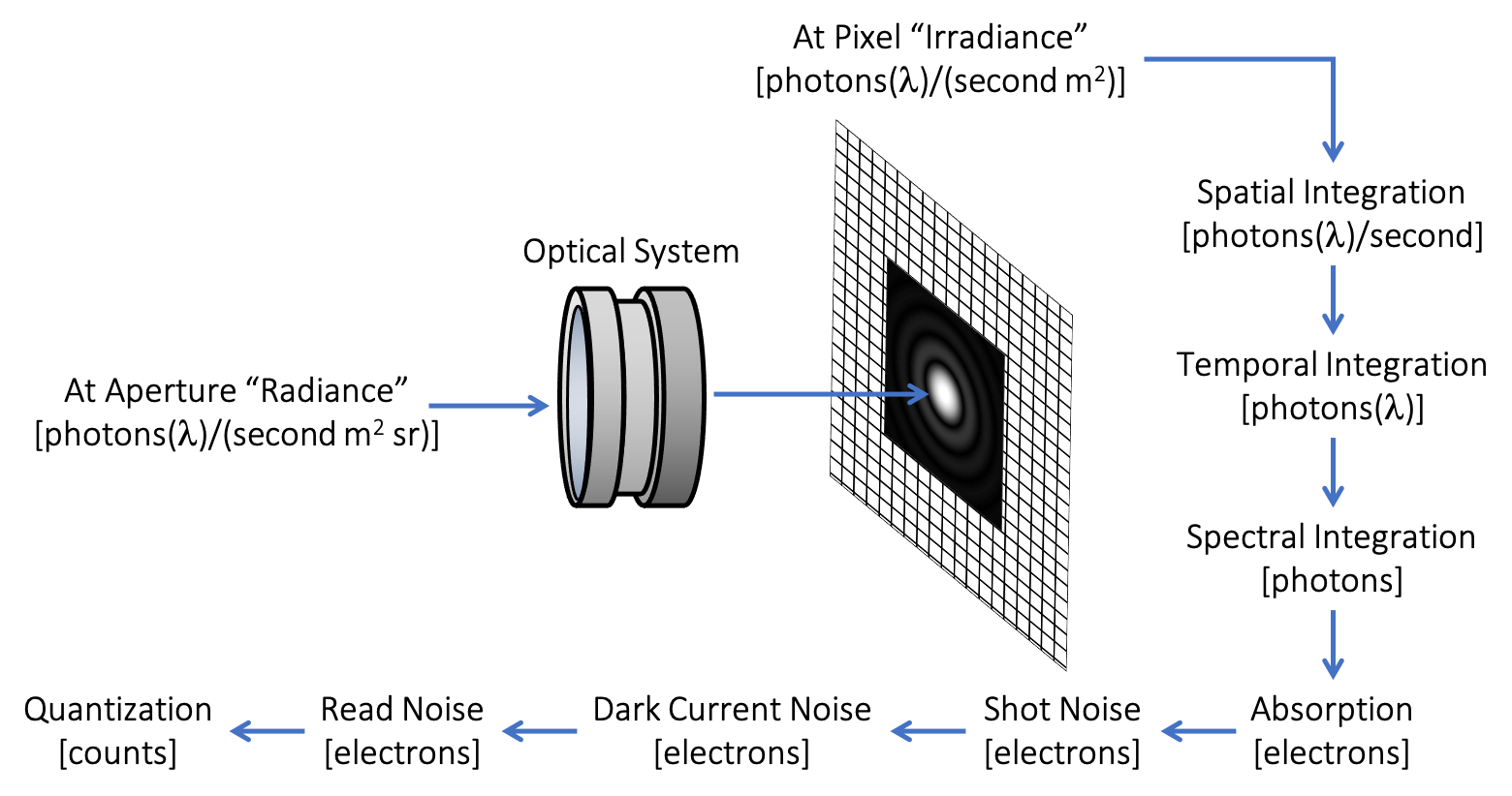
For users that do not wish to perform this modeling externally, the internal detector model described here provides the user with the option to produce output data that is in digital counts and features Shot (arrival) noise, dark current noise, read noise and quantization. The general flow of the calculations is as follows:
-
The at aperture spectral radiance [photons/(s cm2 sr)] is propagated through a user-defined, clear aperture to compute the at pixel spectral irradiance [photons/(s cm2)].
-
The area of the pixel is used to compute the spectral photon rate onto the pixel [photons/s].
-
The integration time of the pixel is used to temporally integrate how many photons arrive onto the pixel [photons].
-
The channel relative spectral response (RSR) and a user-define scalar quantum efficiency (QE) is used to convert the spectral photon arrival rate into the number of electrons generated in the pixel [electrons].
-
Dead or "hot" pixels are skipped, resulting in either no signal (DC = 0) or maximum signal (DC = max DC), respectively.
-
Shot noise is added using a Poisson distribution with a mean of the number of electrons [electrons].
-
Dark current noise is added using a Poisson distribution with a mean of the number of electrons [electrons].
-
Read noise is added using a Poisson distribution with a mean of the number of electrons [electrons].
-
The number of electrons is scaled using a user-defined analog-to-digital converter (ADC) to produce a digital count (DC).
-
Fixed pattern noise is added to the digital count (DC).
-
The final digital count value is written to the output.
The internal detector model must be configured by manually editing the
.platform file to add the <detectormodel> element and few other
elements. The following .platform file excerpt an be used as a template:
        <instrument type="generic" ... >
          <properties>
            <focallength>125</focallength>
            <aperturediameter>0.017857</aperturediameter>
            <aperturethroughput>0.50</aperturethroughput>
          </properties>
          <focalplane ... >
            <capturemethod type="simple">
              <imagefile areaunits="cm2" fluxunits="watts">
                <basename>vendor1</basename>
                <extension>img</extension>
                <schedule>simulation</schedule>
                <datatype>12</datatype>
              </imagefile>
              <spectralresponse ... >
                ...
              </spectralresponse>
              <spatialresponse ... >
                ...
              </spatialresponse>
              <detectormodel>
                <quantumefficiency>0.80</quantumefficiency>
                <readnoise>60</readnoise>
                <deadpixelprobability>0.0001</deadpixelprobability>
                <hotpixelprobability>0.0000</hotpixelprobability>
                <darkcurrentdensity>1e-05</darkcurrentdensity>
                <minelectrons>0</minelectrons>
                <maxelectrons>100e03</maxelectrons>
                <bitdepth>12</bitdepth>
                <fixedpatternnoise axis="0">
                  <minimumcount>48</minimumcount>
                  <maximumcount>128</maximumcount>
                </fixedpatternnoise>
              </detectormodel>
              <temporalintegration>
                <time>0.002</time>
                <samples>10</samples>
              </temporalintegration>
            </capturemethod>
          </focalplane>
        </instrument>
Requirements
-
The capture method type must be
simple. This internal model is not available with the "raw" capture method, which is used to produce spatially and spectrally oversampled data for external detector modeling. -
The aperture size must be provided to compute the acceptance angle of the system in order to compute the at focal plane irradiance from the at aperture radiance. This is specified using the
<aperturediameter>element in the<instrument>→<properties>. The units are meters. -
The focal plane must have temporal integration enabled (a non-zero integration time) in order to compute the total number of photons arriving onto the detectors.
|
|
The areaunits and fluxunits for the <imagefile> are
ignored when the detector model is enabled. These unit
options are automatically set to the appropriate values to
support the calculation of photons onto the detectors.
|
Parameters
The following parameters are specific to the detector model and are defined
within the <detectormodel> element of the focal plane’s capture method.
quantumefficiency-
The average spectral quantum efficiency (QE) of the detectors. This spectrally constant parameter works in conjunction with the relative spectral responses (RSR) of the channel(s) applied to the detectors. The channel RSR might be normalized by area or peak response, hence the name relative responses. This QE term allows the RSR to be scaled to a spectral quantum efficiency. If the RSR curve you provide is already a spectral QE, then set this term to
1.0.
|
|
Don’t forget to account for the gain or bias values that are
defined for each channel. In practice, we suggest not introducing
an additional gain transform and leave the channel gain and bias
values at the default values of 1.0 and 0.0, respectively.
|
deadpixelprobabilityandhotpixelprobability-
The probability of a pixel being "dead" (always produces no signal) or "hot" (always produces maximum signal). The map of dead and hot pixels is produced during the setup. The units are fraction (i.e.,
0.01→ 1%) and the default is0. readnoise-
The mean read noise for all pixels in electrons (units are electrons).
darkcurrentdensity-
The dark current noise as an area density. The use of density is common since it is independent of the pixel area and will appropriately scale as the pixel area is increased or decreased (units are Amps/m2).
<minelectrons>,<maxelectrons>and<bitdepth>-
The analog-to-digital (A/D) converter (ADC) translates the electrons coming off the array into digital counts. Electron counts below the minimum or above the maximum will be clipped to these values. The ADC setup is used to linearly scale the electrons within the specified min/max range into the counts into the unsigned integer range defined by the
<bitdepth>. For the example above, a 12-bit ADC will produced digital counts ranging from0→4095.
|
|
Electron counts below the minimum or above the maximum values defined for the ADC will be clipped to the respective upper/lower value. |
|
|
If the minimum and maximum electrons are set to negative values, the quantization step will be skipped and the output of the simulation will be in units of electrons. |
fixedpatternnoise-
The
axisattribute indicates if this fixed and additive noise is either row aligned (axis="0") or column aligned (axis="1"). A row aligned pattern will feature additive noise that is unique and constant in each row. Theminimumcountandmaximumcountdefine the range of this additive noise in digital counts (DCs), which is randomly generated for the array during setup.
Related Options
-
Once the A/D converter scales the electrons into counts, the pixel values are now integer digital counts rather then floating-point, absolute radiometric quantities. Although those integer values can continue to be written to the standard output ENVI image file as double-precision floating-point values (the default), it is usually desirable to write to an integer format. The
<datatype>element in the<imagefile>can be included to change the output data type to an integer type (see the thedata typetag in the ENVI image header file description).
|
|
The example above has the A/D producing a 12-bit output value and the output image data type was selected to be 16-bit unsigned. In this case, the 12-bit values will be written on 16-bit boundaries. Similarly selecting 32-bit unsigned would write the 12-bit values on 32-bit boundaries. Selecting an 8-bit output would cause the upper 4-bits to be clipped from the 12-bit values. |
Point Spread Function (PSF)
|
|
This feature requires manual editing of the .platform file
because the graphical user interface does not support it.
The feature configuration will be lost of you open and save the
.platform file from the Platform Editor.
|
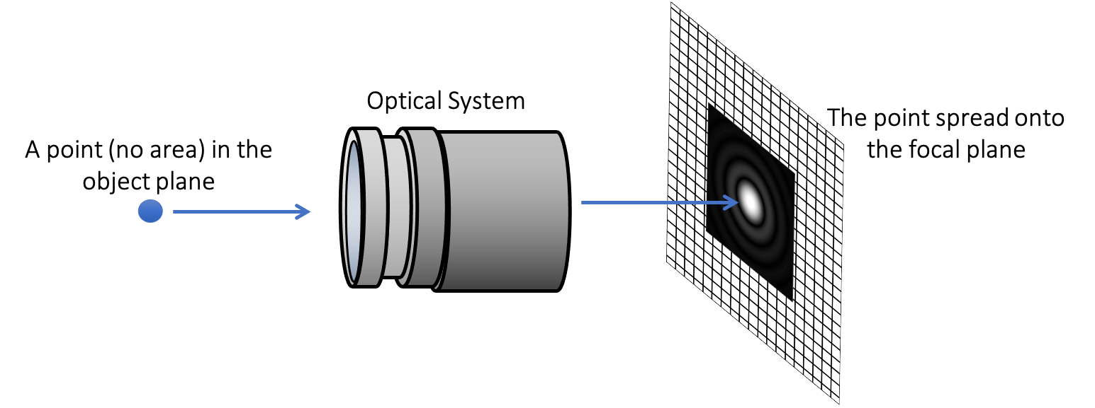
The user can currently describe the modulation transfer function (MTF) of the optical system via a single Point Spread Function (PSF). This function describes the spread of a point (zero area) in the object plane onto the focal plane after passing through the optical system.
Note that a single PSF is provided and hence, this is currently not a position dependent PSF. It should also be noted that the PSF is wavelength constant for the wavelengths captured by the respective focal plane (different PSF configurations can be assigned to different focal planes).
This feature is enabled by manually editing a DIRSIG4 .platform
file and injecting the <psf> XML element in the <focalplane>
element. The PSF is used in a 2-step importance sampling scheme
to emulate the convolution of the PSF with the pixel area. In
general, more samples per pixel are required to faithfully reproduce
the impacts of the PSF on the output. Not that for PSF that is
highly structured and/or very wide (spans many pixels), the maximum
number of paths per pixel might need to be increased (see the
DIRSIG5
manual for details).
Using the built-in Gaussian Profile
For some simple, clear aperture optical systems a Gaussian approximation
of the center lobe of the classic
Airy disk diffraction pattern
is a decent first order solution. For this scenario, the user simply
has to specify the the number of pixels that 1 sigma corresponds to in
the Gaussian shape. In the example below, a Gaussian PSF will be used that
has the 1 sigma width scaled to span 3.8 pixels:
           <focalplane ... >
             <capturemethod type="simple">
               <spectralresponse ... >
                 ...
               </spectralresponse>
               <spatialresponse ... >
                 ...
               </spatialresponse>
               <psf>
                 <width>3.8</width>
               </psf>
             </capturemethod>
             <detectorarray spatialunits="microns">
               ..
             </detectorarray>
           </focalplane ... >
Using a User-Supplied Profile
In this case the PSF is supplied as a gray scale image file (JPG,
PNG, TIFF, etc. via the <image> element) and the user must define
the extent of the image (via the <scale> element) in terms of
focal plane pixels. In the example below, the Airy disk pattern in
the PNG file has an equivalent width of 10 pixels on the focal
plane.
           <focalplane ... >
             <capturemethod type="simple">
               <spectralresponse ... >
                 ...
               </spectralresponse>
               <spatialresponse ... >
                 ...
               </spatialresponse>
               <psf>
                 <image>airy_psf.png</image>
                 <scale>10</scale>
               </psf>
             </capturemethod>
             <detectorarray spatialunits="microns">
               ..
             </detectorarray>
</focalplane ... >|
|
The example above mirrors the setup illustrated in the PSF diagram
at the start of this section. The image file contains the
Airy disk pattern shown as projected onto the focal plane.
The size of that spread pattern captured in the image spans
approximately 10 pixels. Hence, the scale is 10. The
scale is not related to the number of pixels in the PSF
image but rather to the effective size of the pattern in focal
plane pixel units.
|
|
|
Because the PSF effectively increases the sampling area of the pixel, you might need to consider increasing the convergence parameters. The easiest way to explore if this is required for your simulation is to turn on the sample count truth and see if you are regularly hitting the maximum number of paths/pixel (samples/pixel). |
Inline Processing
|
|
This feature requires manual editing of the .platform file
because the graphical user interface does not support it.
The feature configuration will be lost of you open and save the
.platform file from the Platform Editor.
|
There is also an ability to have this plugin launch an external process to
perform operations on the output image. The <processing> element can be
added to each focal plane (inside the <capturemethod> element) and can
include one or more "tasks" to be performed on the supplied schedule.
|
|
Currently these processing tasks are applied to the radiometric image product and not the truth image product. |
The schedule options include:
collection_started-
A processing step that is performed on the radiometric image file at the start of the collection.
task_started-
A processing step that can be performed on the radiometric image file at the start of each task.
capture_started-
A processing step that can be performed on the radiometric image file at the end of each capture.
capture_completed-
A processing step that can be performed on the radiometric image file at the end of each capture.
task_completed-
A processing step that can be performed on the radiometric image file at the end of each task.
collection_completed-
A processing step that can be performed on the radiometric image file at the end of the collection.
|
|
The processing schedule is most likely related to the output file
schedule for the focal plane. For example, if the focal plane
produces a unique file per capture, then the processing schedule
would most likely be capture_completed so that it can perform
post-processing on the file just produced by the capture event.
|
Demosaicing Example
The example below is meant to demonstrate how a (fictitious) program
called demosaic can be run at the end of each capture. The options
(provided in order by the <argument> elements) are specific to the
program being executed:
           <focalplane ... >
             <capturemethod type="simple">
              <spectralresponse ... >
                ...
              </spectralresponse>
              <spatialresponse ... >
                ...
              </spatialresponse>
              <imagefile areaunits="cm2" fluxunits="watts">
                <basename>truesense</basename>
                <extension>img</extension>
                <schedule>capture</schedule>
              </imagefile>
              <processing>
                <task schedule="capture_completed">
                  <message>Running demosaic algorithm</message>
                  <program>demosaic</program>
                  <argument>--pattern=truesense</argument>
                  <argument>--input_filename=$$IMG_BASENAME$$.img</argument>
                  <argument>--output_filename=$$IMG_BASENAME$$.jpg</argument>
                  <stdoutfilename>demosaic_log.txt</stdoutfilename>
                  <removefile>true</removefile>
                </task>
              </processing>
             </capturemethod>
</focalplane>|
|
An <argument> must be a single argument and cannot
contain any whitespace.
|
The special string $$IMG_BASENAME$$ represents the radiometric image
file being generated. In this example, the <imagefile> indicates
that a file with the basename of truesense and a file extension
of .img will be produced for each capture, resulting in filenames
such as truesense_t0000-c0000.img, truesense_t0000-c0001.img,
etc. When this processing task is triggered after the first capture,
the $$IMG_BASENAME$$ string will be replaced by the string
truesense_t0000-c0000. Subsequent processing calls will be
automatically called with the appropriate filename that is changing
from capture to capture.
The <stdoutfilename> and <stderrfilename> options can be supplied
with the name of unique files that will capture the output of the
processing task. These options can be useful for debugging issues with
your processes. Note that since processing tasks typically run multiple
times during a DIRSIG execution, the output from your tasks will be
appended to these files.
The <removefile> option allows you to request that the current file
produced by DIRSIG be removed after the processing task is complete.
In the case of the example above, after the DIRSIG image has been
demosaiced, the original mosaiced image could be removed (to save
disk space, etc.). Note that the ENVI header file will be removed
as well. The default for this option is false.
The <stdoutfilename> and <stderrfilename> options can be set to
route the output of process to separate files so that this output can
be used or reviewed at the end of the simulation. For processing tasks
that are repeated (per capture, per task, etc.) the output is appended
to the files during the simulation.
|
|
These processing steps can also be used to perform tasks unrelated to image data processing. For example, to append the current time into a log file, to perform file housekeeping tasks, etc. The intention is for any program that can be executed from the command-line to be triggerable as part of the simulation event schedule. |
Video Encoding Example
For a more complex example, consider wanting to automatically generate a video file from a simulation. In this example, we will use the ffmpeg utility to encode a sequence of individual frames into a video. To achieve this, we will use the "file per capture" output file schedule (to produce a separate image file for each capture frame) and then define two processing tasks:
-
At the end of each capture, the output file will be converted to a PNG image. In this case we will use the DIRSIG supplied image_tool utility.
-
At the end of the data collection (simulation), all the individual frames will be encoded by the
ffmpegutility (note that the details of theffmpegoptions are beyond the scope of this discussion).
              <processing>
                <task schedule="capture_completed">
                  <message>Converting radiance image to PNG</message>
                  <program>image_tool</program>
                  <argument>convert</argument>
                  <argument>--gamma=1</argument>
                  <argument>--format=png</argument>
                  <argument>--output_filename=$$IMG_BASENAME$$.png</argument>
                  <argument>$$IMG_BASENAME$$.img</argument>
                  <removefile>true</removefile>
                </task>
                <task schedule="collection_completed">
                  <message>Encoding frames into video</message>
                  <program>ffmpeg</program>
                  <argument>-y</argument>
                  <argument>-framerate</argument>
                  <argument>15</argument>
                  <argument>-i</argument>
                  <argument>demo-t0000-c%04d.png</argument>
                  <argument>video.mp4</argument>
                  <stderrfilename>ffmpeg_log.txt</stderrfilename>
                </task>
</processing>|
|
The ffmpeg program writes most of it’s output to standard error
rather than standard output, hence the use of the <stderrfilename>
to capture the output.
|
While the simulation is running, the <message> will be displayed when
each processing task is executed:
Running the simulation
Solar state update notification from 'SpiceEphemeris'
    66.237 [degrees, declination], 175.141 [degrees, East of North]
Lunar state update notification from 'SpiceEphemeris'
    70.153 [degrees, declination], 137.883 [degrees, East of North]
    0.089 [phase fraction]
Starting capture: Task #1, Capture #1, Event #1 of 21
    Date/Time = 2008-12-30T12:00:00.0000-05:00, relative time = 0.000000e+00
    Instrument -> Focal Plane
        Bandpass = 0.400000 - 0.800000 @ 0.010000 microns (41 samples)
        Array size = 320 x 240
Converting frame to PNG
Removing file 'demo-t0000-c0000.img'

...

Starting capture: Task #1, Capture #21, Event #21 of 21
    Date/Time = 2008-12-30T12:00:05.0000-05:00, relative time = 5.000000e+00
    Instrument -> Focal Plane
        Bandpass = 0.400000 - 0.800000 @ 0.010000 microns (41 samples)
        Array size = 320 x 240
Converting frame to PNG
Removing file 'demo-t0000-c0020.img'

Encoding frames into video
An example of this video encoding scenario is included in the
TrackingMount1 demo
(see the encode.platform and encode.sim files).
Focus Distance
This sensor plugin is typically used to model a camera that is
focused at inifinity, where all rays pays through a single focus
point. However, the user can optional specify a finite focus
distance in a camera modeled by the plugin, which triggers an
advanced sampling of the user-defined aperture. The variable that
enables this feature is the <focusdistance> in the instrument’s
<properties> element. In order to enable this feature, the
<aperturediameter> must also be defined.
        <instrument name="RGB Instrument" type="generic">
          <properties>
            <focallength>80</focallength>
            <focusdistance>1.9</focusdistance>
            <aperturediameter>0.072</aperturediameter>
</properties>|
|
The <focallength> parameter is in millimeters, but the
<focusdistance> and <aperturediameter> is in meters.
|
A working example of this feature is provided in the FocusDistance1 demo.
FocusDistance1 demo.Usage
The BasicPlatform is implicitly used when the user launches DIRSIG5
with a DIRSIG4 era XML simulation file (.sim). To explicitly use
the BasicPlatform plugin in DIRSIG5, the user must use the newer JSON
formatted simulation input file (referred to a JSIM
file with a .jsim file extension):
.jsim equivalent of a DIRSIG4-era .sim file.[{
"scene_list" : [
{ "inputs" : "./demo.scene" }
],
"plugin_list" : [
{
"name" : "BasicAtmosphere",
"inputs" : {
"atmosphere_filename" : "mls_dis4_rural_23k.atm"
}
},
{
"name" : "BasicPlatform",
"inputs" : {
"platform_filename" : "./demo.platform",
"motion_filename" : "./demo.ppd",
"tasks_filename" : "./demo.tasks",
"output_folder" : "output",
"output_prefix" : "test1_",
"split_channels" : false,
"scene_index" : 13
}
}
]
}]Options
Output Folder and Prefix
DIRSIG4 and DIRSIG5 support a common pair of
options to specify the output
folder and/or prefix of all files generated by the sensor plugins.
The optional output_folder and output_prefix variables serve
the same purpose as (and take precedence over) the respective
command-line --output_folder and --output_prefix options. The
value with providing these options in the JSIM file is that each
BasicPlatform plugin instance can get a unique value for these
options, where as the command-line options will provided each plugin
instance with the same value.
For example, consider a simulation with multiple instances of the
exact same sensor flying in different orbits (e.g., a constellation
of satellites). The constellation can be modeled in a single
simulation using multiple instances of the BasicPlatform plugin,
each being assigned the same .platform file but a different
.motion file with the unique orbit description. Since each
instance is using the same .platform, each instance will write
to the same output files. Using the output_prefix (or the
output_folder) option in the JSIM allows each instance to generate
a unique set of output files while sharing the same platform file.
[{
    "scene_list" : [
        ...
    ],
    "plugin_list" : [
        ...
        {
            "name" : "BasicPlatform",
            "inputs" : {
                "platform_filename" : "./my_sat.platform",
                "motion_filename" : "./sat1.motion",
                "tasks_filename" : "./sat1.tasks",
                "output_prefix" : "sat1_"
            }
        },
        {
            "name" : "BasicPlatform",
            "inputs" : {
                "platform_filename" : "./my_sat.platform",
                "motion_filename" : "./sat2.motion",
                "tasks_filename" : "./sat2.tasks",
                "output_prefix" : "sat2_"
            }
        }
    ]
}]
Split Channels into States
By default, this plugin submits the bandpass for each focal plane as a separate spectral state to the DIRSIG5 core. That means that a single wavelength will be used to geometrically follow light paths through the scene. This approach is fine unless spectral dispersion (e.g., refraction separating different wavelengths) is expected or desired. For example, if a single focal plane is assigned red, green and blue channels and the user expects atmospheric refraction to create spectral separation, then the single spectral state approach will not work because a single, common wavelength will be used to compute the refraction for red, green and blue light. The first alternative is to create multiple focal planes, which will result in each submitting a unique spectral state and as a result different wavelengths will be used to compute the refraction for each channel.
|
|
On average, atmospheric refraction can be significant, but the relative differences between channels in a single camera is usually minimal except at severe slant angles (low elevation) an long path lengths. The Refraction1 demo contains an example this effect in practice. |
The second alternative is the "split channels into states" option,
which forces the plugin to submit a unique spectral state for each
channel in each focal plane. The optional split_channels variable
in the JSIM input serves the same purpose as (and takes precedence over)
the respective command-line --split_channels option. The default
is false.
Scene Index
The (optional) scene_index variable can be specified in cases
where the platform motion (either a GenericMotion
.ppd or FlexMotion .motion file) has
scene-relative (Scene ENU) coordinates
and there are multiple scenes in the
simulation. This variable defaults to 0, which corresponds to the
first scene loaded. If the user wants to make the Scene ENU motion
relative to a different scene, then the scene_index variable should
be set to the index for that scene.
|
|
The scene indexes are printed to the output when DIRSIG is run and/or can be foudn via the scene index truth. |
Scale Resolution
In some situations, the user may want to modify a focal plane to
get a higher resolution (more pixels) or lower resolution (fewer
pixels) image of the same field-of-view (FOV). This can be manually
achieved by modifying the geometric camera model via the pixel
sizes, number of pixels, etc. An easier alternative is the "scale
resolution" option, which allows the user to quickly change the
resolution. The command-line --scale_resolution option is assigned
a resolution scaling factor (e.g., --scale_resolution=2.0). The
default value is 1 but providing a factor > 1 will increase the
resolution (more pixels) and a factor < 1 will decrease the
resolution (fewer pixels). This factor will be applied to all
the focal planes in all the instruments modeled by this plugin.