|
|
This document is currently under construction. |
This document discusses the details of using the DIRSIG image and data generation model to simulate Radio Detection and Ranging (RADAR) systems.
Overview
History
The initial version of the DIRSIG radar capability were created during the developement of 4.2 releases as a stand-alone application that leveraged the DIRSIG core libraries. During the 4.3 development cycle this proof of concept tool was integrated within the main DIRSIG application and internal experimentation continued. At this time, the capability was still an unfunded project being conducted during off hours. During the 4.4 releases a set of minimal demos were created in an effort to obtaining funding for focused development. Closer to the end of the 4.5 release cycle the first version of this document was produced in an effort to help users play with the tool and provide feedback. The 4.6 release brought improvements to the scene and platform descriptions and a major refreshment of the demos.
Technical Readiness
This application area is currently ranked as experimental due to the lack of some key features and lack of extensive use by RIT and the user community.
Model Strengths
-
Ability to model real aperture radar (RAR) and synthetic aperture radar (SAR) systems.
-
Direct output of complex Phase History data
-
Rather than directly produce radar imagery, the model’s primary output is the complex signal return. This allows the user to test complex collection scenarios and processing algorithms to "focus" those phase histories into imagery.
-
-
Optional pulse compression via linear frequency modulation (LFM)
-
Quad-polarization capable (HH, HV, VH and VV)
-
Bi-static transmit and receive options
-
Platform motion (programmed and unprogrammed (jitter) motion) and platform-relative dynamic pointing (and scanning) allow the user to model common SAR collection modes:
-
Stripmap (constant beam forming to map a large area)
-
Scan (beam steering to scan a small area)
-
Spotlight (beam steering to stare at an even smaller area)
-
-
Detailed scenes, material variations and in-scene motion
-
Doppler effects can be enabled to model moving target indicators (MTI)
-
Model Weaknesses
-
Atmospheric attenuation (absorption) is not model driven
-
The MonoRTM line-by-line atmospheric radiative transfer model can be used to compute transmission impacts from dominant atmospheric absorbers in the RF region (oxygen, water vapor and water droplets).
-
-
Phased array systems are not directly modeled
-
The user must utilize the platform orientation or platform-relative pointing to emulate beam steering effects.
-
-
Spectral bandwidth is not currently modeled. Only the central carrier frequency is currently used in the radiometry.
-
Interfaces to facilitate user-defined frequency and phase modulation schemes are not available
-
We would like to enhance the model to allow the user to describe the beam shape, carrier frequency, chirp segments, etc. on a per-pulse basis. This would allow the end user to model nearly arbitrary modulation schemes including step chirp, binary-phase coding, polyphase coding, etc.
-
-
RF noise is not modeled
-
A limiting factor on detection is the signal-to-noise ratio in the receiver. The spectral bandwidth of the receiver can, therefore, dictate how much noise is received while listening for an echo.
-
The existence of these limitation is primarily a result of funded research priorities. Our past and current research has not placed a priority on resolving this current set of limitations. As researchers, we are always seeking opportunities to to address known limitations if funding is available.
Technical Background
A RADAR system emits radio frequency (RF) pulses from a location and measures the time it takes for them bounce off objects and return. This travel time can then be used to compute the distance or range to the object(s) that reflected the pulse back to the system. Single-pulse data is usually visualized as a 1D intensity vs. time or intensity vs. range. Imaging radar systems map 2D regions by sending multiple pulses and scanning via either platform or antenna motion. For example, most airport (tracking) and weather radars scan by rotating the antenna. In contrast, most airborne radar systems shoot pulses to measure intensity vs. range information in the across-track direction while the movement of the aircraft is used to scan the along-track direction. A radar system can employ a single antenna that is employed for both transmitting and receiving signals (a duplexer will switch the antenna between the transmitter and receiver), or employ separate antennas for each task. Some systems have transmit and receive antennas that are spatially separated (a bi-static configuration).
There are are many factors that limit the spatial (range) resolution of a radar system. A Synthetic Aperture Radar (SAR) uses a smaller antenna in conjunction with a time-multiplexed approach to mimic the aperture (and resolution) of a larger antenna. In order to synthesize the larger apparent aperture, the knowledge of the platform’s location and orientation must be well known. Knowledge errors (for example, assuming a flight is perfectly straight when there was a lot of jitter) will lead to defocusing of the final image product because the backprojection will place intensity information into the wrong range bins.
A generalized antenna is usually characterized by (a) the gain, which is usually proportional to the area and efficiency of the antenna and (b) the directionality (or directivity), which is characterized by the width of the beam at some magnitude (for example, the angular width at 3 dB). Basic antennas can utilize a simple dipole configuration. Early designs would sometimes combine multiple dipoles to achieve directionality. Later, parabolic reflectors were coupled to a central feed in order to increase the gain and directionality of the beam. Advanced radar systems employ multiple antennas, which can be phased in order to steer the beam in a given direction.
Transmitter Characteristics
A radar typically emits pulses at a constant pulse repetition frequency (PRF). This might also be described in terms of the pulse repetition interval (PRI) or the pulse repetition time (PRT). The length of a pulse is referred to as the pulse width (PW) in seconds. Each pulse last for a short fraction of the period between pulses, and the duty cycle refers to the fraction of the total time during which the transmitter is emitting energy. For example, if the pulse repetition interval is 100 microseconds and each pulse is 1 microsecond long, then the duty cycle is 1%. Most temporal pulse profiles are approximated as a RECT function (infinite slope on the rise and fall), but are less ideal in reality.
The spectral distribution of the emitted pulse is typically characterized in terms of a central carrier frequency and a spectral bandwidth about that frequency. Most airborne and space-borne imaging real aperture radar (RAR) and synthetic aperture radar (SAR) systems operate in the X Band or the 8.0 - 12.5 GHz (2.4 - 3.75 cm wavelength) range. Like the temporal pulse width, the spectral bandwidth is usually approximated as a RECT function, but the actual frequency envelope is usually less ideal.
Pulse Compression
The concept of pulse compression is to manipulate the temporal characteristics of the transmitted pulse shape (profile) in order to achieve improved range resolution and/or noise rejection. There are generally two classes of schemes commonly employed:
-
Frequency Modulation (FM)
-
Linear Frequency Modulation (LFM) or "chirp" modulation involves linearly modulating the signal with frequency. A matched filter (using the chirp) is then employed in the receiver to isolate returns. LFM is common pulse compression method because the hardware implementation is not complex (a bank of delay lines can be used). However, sidelobes are present that must be amplitude weighted (windowed) to improve the match filter performance, which can lower the signal-to-noise.
-
Non-Linear Frequency Modulation (NLMF) methods attempt to produce compressed waveforms with dramatically lower sidelobes. This means that amplitude weighting can be avoided and signal-to-noise can be preserved. However, NLFM systems are more complex to implement in hardware.
-
-
Phase Modulation (PM)
-
Phase modulated or phase coded methods break the transmitted pulse into a series of short (sub) pulses that are typically equal in length. Each sub-pulse is generally mapped to a given range and is assigned a specific phase. These sub-pulse phase sequences (codings) are then used to improve from what range a response was generated.
-
|
|
At this time the DIRSIG model only supports Linear Frequency Modulation (LFM) pulse compression. |
Receiver Characteristics
This section will eventually describe the receiver in greater detail. For now, the receiver is assumed to have the same angular sensitivity as the transmitter. The key receiver characteristic is the range gate (temporally listening window).
Implementation Details
We should then have a section describing the details of the numerical approach (implementation) of the radiometric solution. This section should outline the ray tracing and geometry sampling approach to support coherent detection.
Two-Stage Simulation Approach
Similar to the approach employed for the LIDAR Modality, we employ a two stage approach for RADAR:
-
A radiometry stage, where pulses are transmitted, they interact with the scene and they are collected at the receive antenna.
-
An image focusing stage, where the complex receive signal is converted into a traditional radar image.
Note that the primary output of DIRSIG is the raw, complex return data. Although it is our plan to distribute a minimal image focusing tool, the user is required to employ their own algorithm to convert the raw, complex return data into imagery (example Matlab code is included in the demos).
Single vs. Two Pass Radiometry
Within the radiometry stage, you can run the model in either a
single-pass or two-pass mode. In a single-pass radiometry simulation,
the transmit and receive computations are computed during a single
DIRSIG simulation. The output of the simulation is the complex
return. In a two-pass radiometry simulation, the user runs DIRSIG
once to transmit the pulses into the scene and then runs a second
simulation to collect the pulses onto the receiver. The two
simulations are coupled via a storage file (see the twopassmode
and nodefilename variables discussed later).
The benefits of the two-pass method is that the coherent hit map created in the first pass and then used in the second pass results in dramatic reduction in the numerical noise. The noise in the single-pass method arises from random sampling that is different from pulse to pulse. This introduces variations in randomly varying distances to stationary objects between pulses, and manifests itself as random variations in coherence lengths.
|
|
In the future, even the single pass method will employ the coherent hit map approach. |
Atmospheric Modeling
This is where we will outline support for modeling atmospheric effects. Most of our recent simulation work has employed use of the Simple atmosphere model, which lacks the path attenuation from oxygen, water vapor and water droplets (the three dominate absorbers for the radar wavelengths).
Model-Based Atmospheric Modeling
The following model-based atmospheric models can (should) be discussed the future:
-
Using MonoRTM (line-by-line atmospheric RT code) with the Classic atmosphere model.
-
Atmosphere model developed at Sandia National Laboratory (SNL) that accounts for attenuation due to oxygen attenuation, water vapor attenuation, cloud liquid water attenuation, and attenuation due to rain. This model is referred to as the ClassicRF model within the DIRSIG code, but I do not believe we ever added interfaces to use it.
Due to the index of refraction varying vertically and horizontally, the atmosphere can also bend the path of the beam. These effects are not currently accounted for in the SAR calculations, although these calculations have been incorporated into the LIDAR beam propagation.
Scene Modeling
At this time, a DIRSIG radar simulation uses the same scene geometry constructs as an EO/IR simulation. However, a specialized material description model has been added to specifically address the RF wavelength regions encountered in a radar simulation.
Surface Reflectivity Model
A specific reflectivity model was introduced for use exclusively with radar simulations. Although most radar collections usually involve a nearly mono-static transmit and receive geometry, this reflectivity model predicts the bi-directional reflectivity of a surface via a 5-parameter formulation:
\( \mathrm{BRDF}( \theta_i, \theta_o, \Delta \phi ) = d + s \cdot \mathrm{MM}( \theta_n, n, k ) \cdot e^{\frac{-\tan^2 \theta}{2 \sigma^2}} \)
where s and d are the specular and diffuse reflectivity coefficients, respectively, sigma is the surface roughness and n and k is the complex index of refraction which drives the computation of the polarized MM (Mueller Matrix) for the specular component.
|
|
The 5-parameter model is wavelength independent (spectrally constant) at this time. The parameters must be specified for the wavelength (frequency) of the system to be simulated. At a future date support for specifying the parameters as a function of wavelength (or frequency) may be added to allow different systems to be modeled from the same material description. |
In DIRSIG 4.6.x and later, the reflectivity model coefficients are stored in the standard material database file associated with the scene.
|
|
At this time, the material database used with a radar instrument
is specific to a radar simulation. In practice, scenes will most
likely have one configuration which utilizes a standard material
file utilizing the traditional surface properties and radiometry
solvers. There will then be an additional configuration (an
additional .scene file) for radar simulations that uses the
same geometry, but which points to a material database utilizing
radar specific surface property descriptions.
|
The excerpt below shows an example MATERIAL_ENTRY from a DIRSIG material
database file:
MATERIAL_ENTRY {
   ID = 100
   NAME = Ground
   EDITOR_COLOR = 0.5, 0.5, 0.5

   RAD_SOLVER_NAME = Null
   RAD_SOLVER {
   }

   SURFACE_PROPERTIES {
       REFLECTANCE_PROP_NAME = SarReflectivity
       REFLECTANCE_PROP {
           N = 10.00
           K = 4.40
           SIGMA = 0.10
           RHOS = 1.00
           RHOD = 0.00
       }
   }
}
Currently, a radar simulation does not use the same radiometry solver mechanism that the passive and active EO/IR simulations leverage. However, DIRSIG requires that all materials have a radiometry solver assigned to them. The Null radiometry solver allows the material description for a radar simulation to be simplified by specifying a solver that performs no calculations (because it will never be called within the context of a radar simulation).
|
|
The DIRSIG material database editor does not support the setup of these material entries at this time. Therefore, the material database file must be hand-crafted. |
|
|
For radar simulations in DIRSIG releases up to and including
4.5.4, the standard material database file specified in the
.scene file was essentially ignored. Instead, the 5-parameter
reflectivity coefficients for materials were supplied within
the .platform file.
|
Platform Configuration
There are two radar instruments to choose from:
- basic radar
-
This instrument is chosen by specifying the
typeasradar. The returns computed by this instrument are the product of an unpolarized transmitter and receiver setup. The output is a single, complex value for each range bin. - quad-polarized radar
-
This instrument is chosen by specifying the
typeaspolsar. The returns computed by this instrument are the product of a quad-polarized transmitter and receiver setup. The output is four, complex values for each range bin representing the HH, HV, VH and VV polarization combinations.
The setup of either instrument type is otherwise the same. The configuration of the transmitter and receiver are outlined in the following sections. Since this document is still under construction, it is strongly advised to consult the example platform files included with the demos.
|
|
At this time, a radar instrument cannot be combined on a platform with another instrument. |
Transmitter
The transmitter is described via a decomposition of the major characteristics:
-
Spectral
-
The main carrier wavelength
-
The (optional) chirp rate
-
-
Angular
-
The X (range) and Y (azimuth) normalized power distribution
-
-
Temporal
-
The pulse length (seconds) or pulse bandwidth (Hertz)
-
The pulse peak power (Watts)
-
| Variable Name | Description | Units | Notes |
|---|---|---|---|
|
The linear frequency modulation (LFM) chirp rate on the carrier |
Hertz/second |
If set to |
Receiver
The receiver is described via a decomposition of the major characteristics:
-
Range gate description (start, stop and delta)
-
Output complex phasehistory filename
-
The flag to strip (unmix) the carrier frequency
| Variable Name | Description | Default | Notes |
|---|---|---|---|
|
Defines when to when to start and stop the A/D output |
Includes |
Seconds after pulse center leaves transmit antenna |
|
The name of the output file containing the raw, complex data |
(required) |
|
|
Flag to strip (unmix) the carrier frequency in the output |
Default value is false |
|
|
Most of these variables appear in the <receiver> section, but are
conceptually higher level variables shared by the transmitter and
receiver.
|
Modeling Options
The following options are specific to a radar simulation:
-
The number of samples and maximum number of bounces tracked.
-
The coherence length, node quantization value (threshold) and node filename
-
The flag to enable fine motion (Doppler) effects
-
The flag to enable detailed debug messages
-
The flag to use a repeatable transmit seed (to correlate multiple simulations)
| Variable Name | Description | Default | Notes |
|---|---|---|---|
|
The number of photon packets shot from the transmitter |
(required) |
(none) |
|
The maximum number of bounces for each photon packet |
(required) |
(none) |
|
Flag to generate console output during transmit and receive |
false |
(none) |
|
Flag to enable debug output |
false |
(none) |
|
Flag to enable fine motion (Doppler) |
true |
Enables Doppler effects with moving geometry |
|
The name of the node file used for couple two-pass mode |
string |
|
|
The minimum distance between any two coherent sampling points in the scene |
meters |
poor name? |
|
The minimum distance that two points are considered coherent |
meters |
Default seems to work fine for demos |
Example Instrument Description
The following is an example of an <instrument> section of a .platform
file compatible with DIRSIG 4.6.x:
<instrument type="radar" name="RADAR Instrument" >
  <clock type="dependent" temporalunits="hertz">
    <rate>10000</rate>
    <offset>0</offset>
  </clock>
  <transmitter type="pointlaser">
    <spectral shape="gaussian" spectralunits="ghz">
      <center>9.6</center>
      <width>0.0003</width>
    </spectral>
    <spatial shape="rectangular" angularunits="radians">
      <xdivergenceangle>0.01</xdivergenceangle>
      <ydivergenceangle>0.01</ydivergenceangle>
    </spatial>
    <temporal shape="rect" temporalunits="seconds" powerunits="watts">
      <pulseduration type="constant">1.0e-05</pulseduration>
      <pulsepower type="constant">1.0e+09</pulsepower>
    </temporal>
    <modulation type="linearfreq">
      <chirprate>2.506e+13</chirprate>
    </modulation>
  </transmitter>
  <receiver>
    <signalgate temporalunits="seconds">
      <min>1.335e-04</min>
      <max>1.495e-04</max>
      <delta>2.0e-08</delta>
    </signalgate>
    <stripcarrier>0</stripcarrier>
    <imagefilename>sar.img</imagefilename>
  </receiver>
  <options>
    <samples>250000</samples>
    <maxbounces>3</maxbounces>
    <enabledebugoutput>0</enabledebugoutput>
    <enableverboseoutput>1</enableverboseoutput>
    <nodemapfile>hit_nodes.dat</nodemapfile>
    <nodemergeradius>0.5</nodemergeradius>
  </options>
</instrument>
This example employs the "basic radar" (non-polarized) instrument
type. The transmitter emits pulses at a 10 kHz rate with 1.0e+09
Watts (1 GW) continuous power. The pulses have a 9.6 GHz carrier
wavelength (note that the 0.001 spectral bandwidth is ignored at
this time, but the <width> is necessary). The pulses are linear
frequency modulated with a 2.506e+13 Hz/sec chirp rate. The beam
shape is ideal (uniform) with a 0.01 x 0.01 radian (or 10 x 10
mrad) angular width. The transmitted pulse is split up into 250,000
energy packets which are followed for a maximum of 3 bounces.
The pulse-to-pulse coherence hit map employs nodes that will be no
closer than 0.5 meters. The receiver is listening for pulse
returns between 1.335e-04 and 1.495e-04 seconds after a pulse
is fired. The returned signal is digitized with 2.0e-08 second
sampling (50 MHz), which results in 801 (inclusive) range bins.
The output phase history filename will be sar.img and the the
carrier frequency is left mixed in the data (because stripcarrier
is set to 0). The dimensions of the output phase history file
will be 801 x N pixels, where N is the number of pulses shot. This
will be determined by the duration of the collection task and the
10 kHz pulse rate defined here (for example, a 1 second collection
will result in 10000 pulses and the image will be 801 x 10000).
Tx/Rx Beam Steering (Pointing)
In contrast to most EO/IR imaging systems, most radar systems are not oriented to point directly down (nadir) at the scene. Instead, they employ some sort of across-track look angle. This is is handled by orienting the platform, electronic beam steering (via phasing) or a combination of the two. The DIRSIG model does not have have an interface to model a phased array in order to steer the beam at this time. Therefore, the user must rely on platform orientation or platform-relative pointing to direct the beam.
The DIRSIG platform coordinate system has the +Y axis as the nominal along-track axis. Therefore, across-track pointing is rotation about the along-track or Y axis.
There are multiple ways to define the across-track pointing angle:
-
Adding a non-zero Y-axis rotation in the affine transform for the attachment of the instrument to a static mount
-
Defining a non-zero Y-axis rotation in the orientation of a static mount
-
Defining a non-zero Y-axis rotation in the orientation of the platform
Although the final option works just as well as the others, it is less favored because it conceptually implies that the aircraft is flying with a constant roll.
Running Simulations
The preferred simulation approach is the two-pass simulation approach, where a transmit simulation is performed that shoots the radar pulses into the scene and then a receive simulation is performed to receive those pulses back.
|
|
The user can run DIRSIG in a way to perform the transmit and receive calculations within a single simulation. However, that single simulation approach does not currently employ the coherence hit map approach that that the two-pass approach uses to dramatically improves the numerical noise. |
The two-pass mode approach can be enabled at run time using either
an .options file or via a command-line argument (the later is
preferred from a simplicity standpoint).
|
|
The user can also configure a two-pass approach simulation
using the a special flag in the .platform file. However,
this requires separate transmit and receive .platform
files that are identical except for this flag. This also
requires two .sim files which are identical except for
which .platform file is used. This creates extra complexity
and the potential for transmit and receive setups to become
mismatched. Therefore, the command-line option approach
is strongly encouraged.
|
Running the Transmit Simulation
The transmit simulation can be run using the following command-line syntax:
$ dirsig --option="radar.mode=transmit" example.sim
The radar.mode option is what enables the two-pass mode. In this case,
the option was assigned the transmit value to trigger the transmit mode
calculations.
The primary output of the transmit simulation is the hit_nodes.dat file,
which is a special file that records transmit energy packet hit points
within the scene. These are then used in the receive simulation to compute
coherent return intensities.
Running the Receive Simulation
The receive simulation can be run using the following command-line syntax:
$ dirsig --option="radar.mode=receive" example.sim
The output of the receive simulation is a complex phase history, which is described below in detail.
Output
Output Complex Phase History
The output of a DIRSIG radar simulation is the complex signal received by the antenna. This is stored into an output file that is organized as a single band "image" (complete with an ENVI header to visualize it):
-
The X axis (samples) is the "range" axis defined by the number of time bins in the simulation.
-
The Y axis (lines) is the "azimuth" axis defined by the number of pulses fired during the simulation.
-
There is no header data (offset) in the binary data file.
-
The number of bands depends on which instrument is used:
-
For the "plain" radar instrument, there is only 1 band
-
For the "quad-pol" radar instrument, there are 4 bands (one each for HH, HV, VH and VV respectively).
-
-
The band interleave is "band interleaved by pixel" (this is only relevant for the quad-pol SAR instrument which produces 4 output bands).
-
The data type is binary, double-precision, complex data.
For more information on the structure of the output binary data file, look at the DIRSIG image file format document.
|
|
The built-in image viewer cannot display complex image data. To directly visualize the data, you will need to load it in ENVI or implement your own visualization method. |
Output Image Focusing
The complex phase history produced by a DIRSIG SAR simulation must be "focused" into an image. For traditional imaging SAR applications, the focusing algorithm reconciles the returns from all ranges across all pulses to produce an 2D intensity map for the area that was mapped. The details of SAR image focusing algorithms are beyond the scope of this manual but many detailed resources are available. At this time it is expected that most users will be using their own focusing algorithms with the complex phase histories generated by the DIRSIG model. Those algorithms will need access to information that is contained in some of the DIRSIG input/output files:
-
The complex phase history file contains the input data to be processed.
-
The Imaging Platform (
.platformfile) contains important system parameters including the pulse repetition rate (PRF), carrier frequency, modulation rates, etc. -
The Platform Motion (for example, a .
ppdor.motionfile) contains information about the location and orientation of the platform as a function of time (note that a Data Recorder instrument could be used to output this information in an easier to ingest format).
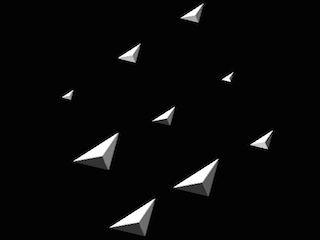
Some of the DIRSIG demos include a Matlab focusing algorithm based on the work of Gorham and Moore. The example below shows an array of corner (trihedral) reflectors and an animation of the focused intensity image as the algorithm incorporates new intensity vs. range information from each pulse.
Demonstrations
This section should list the demos we have available and a brief description of what they cover. The current list includes:
- StripmapSar1
-
A "stripmap mode" collection over an array of corner (trihedral) corner reflectors. This demo includes Matlab code to focus the raw, complex data into an image.
- SpotlightSar1
-
A "spotlight mode" collection staring at an array of corner (trihedral) corner reflectors. This demo includes Matlab code to focus the raw, complex data into an image.
The Roadmap
The SAR capability in the DIRSIG model needs a significant amount of work to bring it in line with the production level capabilities of the other modalities. The following sections highlight a subset of items that need to be addressed to mature this capability.
Technical To-Do Items
This section outlines the short-term, technical tasks required to get this capability out of the "experimental" phase.
-
The single-pass and two-pass method should both use the coherent hit map approach.
-
The un-pol and quad-pol SAR instruments should be unified to use the same code except for the final contribution calculation, which would address un-pol vs. quad-pol aspects.
-
Create a basic graphical user interface so the user can setup and manipulate the radar instrument (rather than hand-edit the
.platformfile). -
Work on output file meta-data embedding
-
Develop a "standard" focusing tool that works with the embedded meta-data output files.
-
Add a moving target (Doppler) demo.
Documentation To-Do Items
-
Do we assume the receive antenna has the same angular sensitivity as the transmitter? Should we add the option of a receiver specific angular sensitivity?
-
We need to make a detailed document for what the file format looks like when we embed this meta-data. Something like the BIN file document is a great template.
-
We don’t discuss how to setup a bi-static system.
Future Directions
Once the current modeling capabilities have been cleaned up and stabilized, the next step involves the addition of an advanced, data-driven mechanism that would allow users to model advanced systems. The primary goal of this effort would be providing a mechanism to drive the transmitter on a pulse by pulse basis. This would allow the user to describe the beam shape, carrier frequency, chirp segments, etc. on a per-pulse basis. This would allow the end user to model nearly arbitrary modulation schemes including step chirp, binary-phase coding, poly-phase coding, etc. Furthermore, allowing for multiple transmitters and per-transmitter pulse descriptions like those previously described would allow phased array systems (beam steering) to be directly modeled (currently the user can have only a single transmitter and beam steering must be accomplished with platform orientation or platform-relative pointing).
References
LeRoy A. Gorham and Linda J. Moore, "SAR image formation toolbox for MATLAB", Proc. SPIE 7699, Algorithms for Synthetic Aperture Radar Imagery XVII, 769906 (April 18, 2010).
Michael Gartley, Adam Goodenough, Scott Brown and Russel P. Kauffman, "A comparison of spatial sampling techniques enabling first principles modeling of a synthetic aperture RADAR imaging platform", Proc. SPIE 7699, Algorithms for Synthetic Aperture Radar Imagery XVII, 76990N (April 18, 2010)
Armin W. Doerry, "Atmospheric loss considerations for synthetic aperture radar design and operation", Proc. SPIE 5410, Radar Sensor Technology VIII and Passive Millimeter-Wave Imaging Technology VII, 17 (August 12, 2004)
John A. Richards, "Simulating the effects of long-range collection on synthetic aperture radar imagery", Proc. SPIE 7337, 73370E (2009).