Summary
The LightCurve plugin is a sensor plugin that was created to allow users to quickly generate a 1D (magnitude vs. time) light curve datasets. The traditional application of light curves is in observing the modulations of distant stars, however the space domain awareness (SDA) community have been using light curves to characterize orbiting assets including active satellites and space debris.
The LightCurve sensor plugin works by automatically tracking the
indicated target object using the supplied geometry tag (in this
case, seasat1). The user supplies a start date/time and duration
for the desired data collection. For each time step during the
collection, the field-of-view (FOV) that encompases the extent of
the tracked object is sampled using a M x M sample grid. The samples
are spectrally and spatially integrated to produce a total integrated
radiance, which is also converted to a magnitude (commonly used for
light curves).
Input
Scene Requirements
The plugin will automatically track compute the radiance (and visual
magnitude) of a specified object as a function of time. The object
to be measured is indicated using a geometry tag
associated with an object in the simulation. This is usually achieved
by introducing a tag to an instance in a GLIST file. See the seasat1
tag on the dynamic instance for the SeaSat-1 satellite in the example
GLIST below:
<geometrylist enabled="true">
  <object>
    <basegeometry>
      <obj><filename>seasat1.obj</filename></obj>
    </basegeometry>
    <dynamicinstance tags="seasat1">
      <motion type="flexible">
        <locationengine type="sgp4">
          <data source="internal">
            <tle1>1 10967U 78064A   23320.39076064  .00000335  00000-0  13623-3 0  9992</tle1>
            <tle2>2 10967 107.9972 156.5508 0001869 301.4908  58.6055 14.44619060384514</tle2>
          </data>
        </locationengine>
        <orientationengine type="lookat">
          <locationengine type="fixed">
            <location type="ecef">
              <x>0.0</x><y>0.0</y><z>0.0</z>
            </location>
          </locationengine>
        </orientationengine>
      </motion>
    </dynamicinstance>
  </object>
</geometrylist>
Atmosphere Requirements
For a terrestrial sensor looking up at an exo-atmospheric object, the atmosphere can contribute to the observed radiance through atmospheric path transmission loses and path scattered and self-emitted radiance contributions. At this time, the MODTRAN-driven NewAtmosphere and FourCurveAtmosphere plugins cannot be used with the LightCurve sensor plugin. This will be resolved in future updates, but for now the user is encouraged to use the SimpleAtm option provided by the BasicAtmosphere plugin.
Plugin Configuration
Rather than construct a carefully crafted platform file for use with the BasicPlatform plugin and employ post processing to produce the light curve, the LightCurve plugin provides a streamlined method to collect and output the desired data.
The input configuration for this plugin is a JSON formatted document. An example is shown below:
{
    "name" : "LightCurve",
    "inputs" : {
        "sensor_location" : {
            "latitude"  : 35,
            "longitude" : -106.0,
            "altitude"  : 0
        },
        "bandpass" : {
            "units"   : "angstroms",
            "minimum" : 5070,
            "maximum" : 5950,
            "delta"   : 1
        },
        "target_tag" : "seasat1",
        "date_time" : "2023-11-16T12:47:00.0000-00:00",
        "duration" : 840,
        "sample_count" : 100,
        "grid_size" : 128,
        "output_filename" : "seasat1_lightcurve.txt",
        "debug_filename" : "debug.grid",
        "image_basename" : "cube"
    }
}sensor_location(required)-
The location of the observation as a latitude (degrees, +N), longitude (degrees, +E) and altitude (meters, WGS84).
bandpass(required)-
The spectral bandpass for the output image to be created. At this time
microns,nanometersandangstromunits are supported. target_tag(required)-
A geometry tag associated with the scene object to track.
date_time(required)-
The ISO8601 date/time for the start of the collection.
duration(required)-
The duration of the collection in seconds.
sample_count(optional)-
The number of uniformly distributed time samples across the duration. The default is
100temporal samples. grid_size(optional)-
The number of points in each dimension of the 2D grid used to sample the field-of-view (FOV). The default is
100x100spatial samples. band_zeropoint(optional)-
The zero point for the output visual magnitude. The default value corresponds for Vega in the V band (~5556Å), which is
3.55e-09erg per second per cm2 per Angstrom. output_filename(optional)-
The name of the output ASCII/Text filename. The default is
lightcurve.dat. debug_filename(optional)-
The name of the (optional) ASCII/Text file that can be used to visualize the sub field-of-view (FOV) samples. A non-empty string must be provided for this file to be generated.
image_basename(optional)-
The base name of the (optional) ENVI spatial-spectral data cube image files that will be produced for each time step. A non-empty string must be provided for these files to be generated.
The normal convergence criteria mechanism is used during the data collection. The sub-FOV grid can be thought of as a grid of "pixels" that are each uniformly sampled and converged independently. At the end of the capture, all the "pixels" are combined to produce the total radiance for the FOV. The plot below is a visualization of all the sub-FOV samples for a given time step (capture) for a simulation observing a partially illuminated sphere. Note that the structure of the grid (in this case, the default 100 x 100 grid) is not apparent as each "pixel" is uniformly sampled. The illuminated portion of the sphere shows up as the more densely sampled region (nearing the maximum number of paths/problem defined by the convergence). The background area and shadowed portion of the sphere are less densley samppled (nearing the minimum number of paths/problem defined by the convergence).
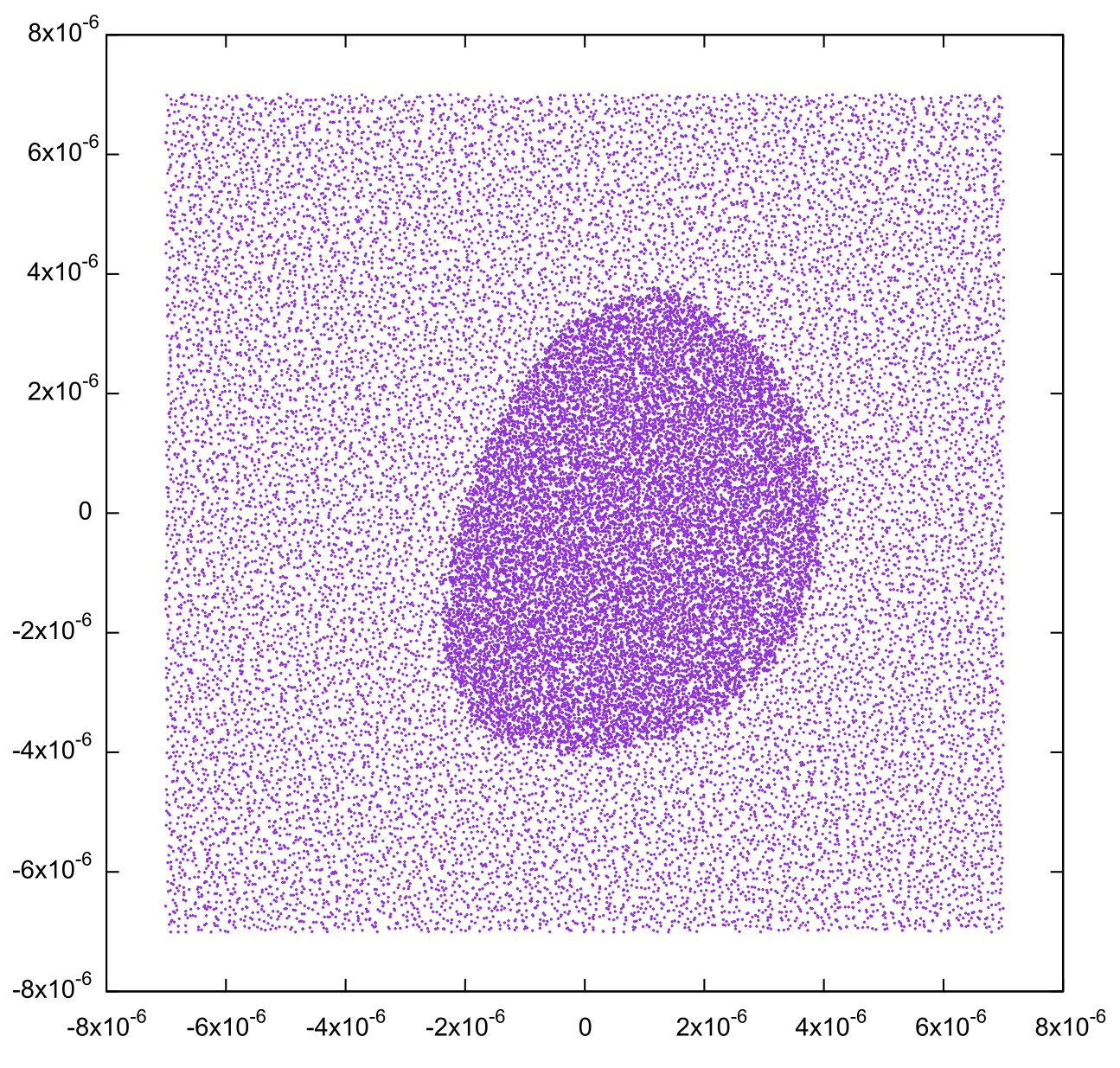
The take-away is that the number of samples per FOV is not the equal to the number of total sub-FOV "pixels". Instead the total number of samples per FOV is the number of sub-FOV "pixels" combined with the minimum and maximum number of samples per "pixel" as defined by the convergence parameters.
|
|
Manipulating the grid_size variable is something that
should only be considered only in extreme scenarios.
Like with most DIRSIG simulations, the convergence
parameters is your primary control over the radiometric
fidelity of the result.
|
Simulation Setup
To use the LightCurve plugin in DIRSIG5, the user must use the newer
JSON formatted simulation input file (referred to a JSIM
file with a .jsim file extension):
[{
    "scene_list" : [
        { "inputs" : "./demo.scene" }
    ],
    "plugin_list" : [
        {
            "name" : "BasicAtmosphere",
            "inputs" : {
                "atmosphere_filename" : "./simple.atm"
            }
        },
        {
            "name" : "LightCurve",
            "inputs" : {
                "sensor_location" : {
                    "latitude"  : 35,
                    "longitude" : -106.0,
                    "altitude"  : 0
                },
                "bandpass" : {
                    "units"   : "angstroms",
                    "minimum" : 5070,
                    "maximum" : 5950,
                    "delta"   : 1
                },
                "target_tag" : "sphere",
                "date_time" : "2023-11-16T12:47:00.0000-00:00",
                "duration" : 840
            }
        }
    ]
}]
In this example, the LightCurve plugin is used with the SimpleAtm model in the Basic Atmosphere plugin.
Output
Primary Output
The primary output of the simulation is a multi-column, ASCII/Text file containing the following values for each time sample:
-
The relative capture time in seconds
-
The magnitude (see note on units and zero point below)
-
The spectrally integrated radiance (Watts per cm2 per steradian)
-
The radius of the bounding volume for the target (in radians), and
-
The solid angle of the bounding volume for the target (in steradians).
The default output filename for the plugin is lightcurve.dat. This
filename can be overridden via the output_filename variable in the
input configuration.
The default zero point for the magnitude is for Vega in the V band (~5556Å)
is 3.55e-09 erg per second per cm2 per Angstrom. This zero point can
be overridden via the band_zeropoint in the input configuration.
4.200000 6.471662e+00 2.760982e-04 2.878857e-06 3.315126e-11
12.600000 6.410562e+00 2.786720e-04 2.947305e-06 3.474643e-11
21.000000 6.349705e+00 2.809153e-04 3.018947e-06 3.645617e-11
...
819.000000 5.712571e+00 1.191655e-03 1.965598e-06 1.545430e-11
827.400000          inf 0.000000e+00 1.934742e-06 1.497291e-11
835.800000          inf 0.000000e+00 1.904844e-06 1.451372e-11
|
|
The 0 value for the radiances and corresponding inf value for
the magnitude indicate that the target was unobservable (below the
horizon) at that time.
|
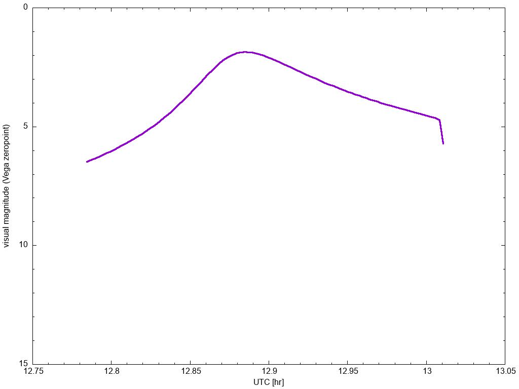
The magnitude vs. time data from the output file is plotted below:
Data Cube Output
If the image_basename was set to a non-zero length string, then
of spatial-spectral data cube image will be produced for each time
step. The spatial dimensions of the images are grid_size x
grid_size. The spectral dimension is the number of wavelengths
in the bandpass. If the image_basename is set to test, then
the resulting image files will be test_000.img, test_001.img,
etc. The number of digits (width) in the numeric sequence portion
of the filename will be sized to hold the number of samples in the
light curve.
|
|
These spatial-spectral data cubes can be used by the user to introduce spectral response weightings for spectral integration, to apply spatial MTFs, to produce temporal-spectral waterfall visualations, etc. |
Debug Output
In some situations it is helpful to visualize the samples within
the field-of-view (FOV) being used to compute the total radiance
(and resulting magnitude) for the FOV of the sensor. For this
purpose, an optional debug "grid file" can be generated during the
simulation (see the optional debug_filename variable in the input
configuration). The FOV was sampled with a M x M uniform grid
(100 is the default, but can be changed via the grid_size
variable). The format of this debug grid file is ASCII/Text, with
each line containing the spectrally integrated radiance for each
of the M samples in a row of the FOV sampling grid. M lines with
M values captures all the samples for a given time. These blocks
of M lines of M values repeats for each time. Hence, a simulation
with N time samples will result in a file with N x M lines and N x
(M x M) samples. Below, these samples for this demo were plotted
and animated as a function of time to show how the solar loading
on the sphere changes as a function of position as it traverses the
sky.
Related Demos
-
The LightCurve1 demo provides a working example of this plugin.