|
|
This guide is a component of the overall Thermal Modality Handbook. |
Introduction
When assigning thermodynamic properties to materials it is useful to consider the way in which each parameter will be used. A link:thermal.html#heat_transfer_basics [general understanding of heat transfer physics] will be useful, and different temperature models may use these properties in different ways. This guide was written with the THERM model in mind, but the thought process can be adapted to any model.
General Insights
A common theme will apply for most thermodynamic properties, materials, and temperature models. Thinking about the temperature prediction from end-to-end will reveal some considerations that are less intuitive than assigning reflective properties. For example, a material might transfer most of its heat into its underlying material and therefore the underlying material might need to be taken into account. For example, a painted concrete material may require the absorptivity and emissivity of the paint to be assigned, while requiring the specific heat and mass density of the concrete. One can reach these conclusions by thinking about the heat transfer process of painted concrete. This guide will point out some of these considerations for each thermodynamic property.
Heat transfer is a subject that has been studied for centuries. As a result, the thermodynamic properties of materials can be found in many physics and engineering resources. It is good practice to reference multiple sources of this information in order to find a consensus. This guide contains some recommended ranges for each THERM property as a result of this procedure. It is possible to encounter errors/outliers when conducting this type of search. If a suspected error is found in one of these resources (including this guide), a quick report of the finding to the resource’s owners is often appreciated.
Thermodynamic Properties
Specific Heat
Specific Heat (C_p) is defined as the amount of energy required to increase one unit mass of a material by one degree. This is clear when looking at the dimensions: J/kg K (or in THERM: cal/g C). When assigning values of C_p for a DIRSIG scene it is important to consider the application. Paint materials, for example, should be assigned C_p values that are representative of the materials the paint is covering, rather than the paint itself. This is because the energy absorbed by the paint will be primarily transferred to the underlying material and any energy storage (or release) as a result of the change in temperature will be affected most by the C_p of the material with more mass. In most applications, the mass of the paint will be orders of magnitude smaller than the mass of the painted material.
|
|
Because the mass is in the denominator of the dimensions, it is important to keep in mind that the density of the material does not affect its specific heat. |
Another factor to keep in mind is that water has one of the highest C_p values in nature. If one type of wood appears in a DIRSIG scene in two different pieces of geometry (e.g. a wooden bench and a boat on a lake), these would contain very different amounts of moisture, drastically changing the C_p. In this case it would be worth duplicating the material and having different sets of thermal properties on each, given the difference in application.
|
|
When assigning materials for plants and other living species, consider the biological processes. For example, the trunk of a living maple tree will contain water and other fluids that will store more heat than a structure made from maple wood. This will require a higher C_p value. |
Thermal Conductivity
Thermal conductivity describes how quickly heat is transferred via conduction. This can be a result of two objects making physical contact, or an object transferring heat internally through a solid material. When assigning thermal conductivity of a material, the context of the scene should be considered. A stained wood material in a desert may conduct heat differently than the same material in a tropical area, for example. The big difference in this example is the moisture content. Many information sources will provide thermal conductivity values for both dry and moist materials when the materials can hold moisture for a long time.
When dealing with mixed materials, the heat conduction of the object should be considered when selecting thermal conductivity values. For example, a type of roofing material that is a near-homogeneous mixture of asphalt with a more thermally insulating material might conduct heat with a weighted average of the thermal conductivities. However, A field with sparse grass and moist soil would likely not be so well behaved and might need to be treated as pure soil when modeling heat conduction.
| Material | Range [ \(\frac{W}{m K}\) ] |
|---|---|
Asphalt |
2.28 - 2.88 |
Brick |
0.6 - 1.0 |
Brick (dense) |
1.6 |
Concrete (low density) |
0.2 - 1.25 |
Concrete (medium density) |
1.25 - 2.25 |
Concrete (high density) |
2.25 - 3.3 |
Glass |
0.96 - 1.05 |
Grass |
2.35 - 2.45 |
Iron |
83 - 70 |
Plastic (acrylic) |
0.2 |
Plastic (HDPE) |
0.5 |
Plastic (PVC) |
0.19 |
Polymers (bulk) |
0.1 - 0.5 |
Polymers (epoxy) |
0.35 |
Rubber (Tire) |
0.13 - 0.16 |
Sand |
0.15 - 0.25 |
Shingle (Roofing Material) |
0.14 - 0.17 |
Steel |
10 - 66 |
Tree Bark (live citrus tree) |
0.41 |
Tree Leaves (live) |
0.26 - 0.57 |
Tree Leaves (dead) |
0.3 - 0.65 |
Wood (Timber) |
0.12 - 0.19 |
Vinyl |
0.12 - 0.25 |
Mass Density
In THERM, mass density is used to calculate the thermal mass of the material. Thermal mass, combined with specific heat, tells THERM how much energy is required to change the temperature of the object. Similar to specific heat and thermal conductivity, mass density should be considered for the bulk of the object rather than the surface alone. A good example of this is a road that is painted with two different colors: white and blue. One would expect the temperature of the white painted road to be slightly cooler than the blue painted road, especially if lateral conduction is ignored. The mass density of the paints themselves matters very little in this situation. The layer of paint on the road contributes very little mass to this heat transfer problem and should be ignored. Instead, the mass density of the asphalt should be considered. In this case, the two road paint materials should be assigned the same mass density values since they are being painted onto the same road. The differences in the other THERM variables will induce differences in the thermal calculation, which should result in the temperature differences mentioned above.
| Material | Range [ \(\frac{g}{cm^3}\) ] |
|---|---|
Aluminum |
2.7 |
Asphalt |
2.2 - 2.4 |
Brick |
1.4 - 2.4 |
Concrete (low density) |
2.28 |
Concrete (medium density) |
2.4 |
Concrete (high density) |
2.55 |
Grass |
2.4 - 2.8 |
Plastic (PVC) |
1.16 - 1.45 |
Rubber (Tire) |
1.1 - 1.2 |
Sand |
1.4 - 1.7 |
Shingle (Roofing Material) |
0.8 |
Steel |
7.82 |
Tree Leaves (live) |
0.1 - 0.6 |
Wood (Timber) |
0.35 - 1.3 |
Thickness
When defining the thickness of a material, the heat transfer throughout the entire object should be considered. Similar to specific heat and thermal conductivity, a coating material such as paint will need the bulk material to dictate the thickness. The thickness of paint on a road may be 1mm or less, but the majority of the heat transfer will occur in the underlying asphalt.
Grass is a particularly interesting material when it comes to defining its thickness. The thickness of a blade of grass might be well known, but may be irrelevant in thermal DIRSIG simulations. The important outcome in a DIRSIG thermal simulation is that the radiance image is correct. The radiance is a function of the "apparent temperature" of the object. When imaging a pixel that is comprised of a patch of grass, there are many factors that affect the apparent temperature of that surface. These factors include grass health, height, growth density, etc. A thick, healthy, tall patch of grass for example will have a surface roughness that decreases the effect the atmosphere has on the ground temperature, however, the pixel would be very representative of the temperature of the grass itself. The opposite is true for a sparse and/or less healthy grass, which would likely behave more closely to the ground material from which it grows. This can lead to very different thickness values for healthy vs. less healthy grass.
There is a maximum thickness in heat transfer problems where adding more thickness will not affect the surface temperature. In heat transfer terminology, an object of this thickness is a "semi-infinite medium". This is useful to keep in mind when defining the thickness of certain terrain materials such as asphalt. The figure below shows this "semi-infinite medium" effect for a few materials. Even if the thickness of the concrete is known, it is appropriate to model it as a thicker asphalt material if the ground below the asphalt is expected to be affected by the surface heat flux.
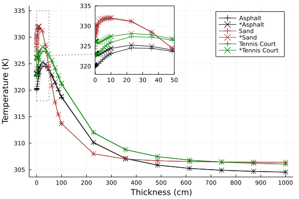
* were defined with negative exposed area.Exposed area
The exposed area term is a scaling factor that tells THERM how much of the surface is exposed to the open sky. In heat transfer terms, the exposed area directly affects the rate of convection caused by the wind. A common scenario is a facet that is flat and exposed to the open sky. Almost any terrain material will fit this description. In this case, an exposed area value of 0.5 should be used. For surfaces that are exposed to the environment on both sides, such as a fence post or a street sign, a negative value (e.g. -0.5) should be used. A value between -0.35 to -0.65 should be used for surfaces that are exposed on both sides. Conversely, surfaces that are exposed on one side should use values between 0.35 and 0.65. As seen in the above figure, exposed area has a diminishing effect as thickness increases.
Optional Parameters
Solar Absorption and Thermal Emissivity
When running THERM, the solar absorption and thermal emissivity terms are calculated using the standard surface optical properties used in DIRSIG. When these properties are explicitly defined under the TEMP_SOLVER entry, these entries will override the mean value calculated by the respective assignment algorithm (spectral emissivity curves, etc.) of the material. This can be useful when the bulk thermal emissivity and/or solar absorption are well known and/or measured for a given material. The texture map and emissivity files will continue to spatially vary the emissivity with the newly defined mean value.
| Material | Range [fraction] |
|---|---|
Asphalt |
0.9 - 0.95 |
Aluminum |
0.9 |
Glass |
0.92 - 0.94 |
Rubber (Tire) |
0.86 - 0.94 |
Sand |
0.8 - 0.92 |
Shingle (Roofing Material) |
0.79 - 0.97 |
Wood (Timber) |
0.88 - 0.95 |