Spherical Quad-Tree (SQT) Manual

DIRSIG4 took an open-ended approach to optical properties — individual models were independently implemented and were only required to respond to basic model queries. This approach was particularly well suited for an academic environment since new models could be brought in directly and easily, often by simply translating equations in papers into code. However, that same open-endedness meant that the level of initialization, general computational complexity, and the potential ability to optimize, varied widely depending on the user’s choice of model. More complex optical property models also needed to be appropriately paired with radiometry solvers that could use the properties as effectively as possible — often requiring fine-tuning of many detailed runtime parameters to achieve both radiometric accuracy and optimal speed.

Our approach in DIRSIG5 was to unify the diversity of optical property model options into a three-prong system. We would provide optimized implementations of "ideal" optical properties (perfectly diffuse, "Lambertian" properties as well as singularly valued or "delta" functions) and a single data-based model to handle everything else. In the development process we added a fourth option to provide an intermediate step above fully diffuse that allows the definition of a specular lobe without having to go all the way to a generic data model for some commonly used, simple models.

As with the models themselves, our approach to optical property radiometry was to replace the various parametrized solvers in DIRSIG4 with a single, unified approach based on Monte Carlo integration. This change means that the quality of radiometry is driven by a single, global parameter (the criteria used to converge to a solution) rather than the myriad solver-specific options that were in place previously.

The data model is a catch-all for any optical properties that are not handled directly with the aforementioned simple analytical models and the way to bring generic optical property data directly into DIRSIG5. The first component of the model is a high spectral resolution integral of the function (i.e. the directional hemispherical reflectance, or DHR), which is stored and handled in a way that is similar to the Lambertian model. The second component is a shaping function that distributes energy into the hemisphere or sphere, i.e. it defines the PDF (probability density function) of the property. It is this function that drives the critical sampling function during a simulation and, in combination with the integral, the direct contribution of sources such as the sun.

A number of different approaches to the PDF model were attempted, including projecting onto basis function representations such as Zernike polynomials and spherical harmonics. However, accurate representation of non-trivial properties required a significant number of coefficients, especially when oscillating on tight lobes that don’t align with the underlying basis functions.

In the end, we decided to take a data-based approach based on a partition of the hemisphere (sphere). The partition is based on the Hierarchical Equal Area isoLatitude Pixelization, or HEALPix, subdivision of the sphere developed by NASA/JPL (https://healpix.jpl.nasa.gov). Each cell of the base, 12 diamond-shaped cell partition over the sphere is successively split into four sub-cells with each depth level step in the hierarchy. The number of cells for a given partition is equal to \( 12 \cdot 4^d\), where d is the depth of the partition. Examples of the parition for depths 3, 4, and 5 are shown below. The corresponding number of cells at each depth are 768, 3072, and 12288, respectively.

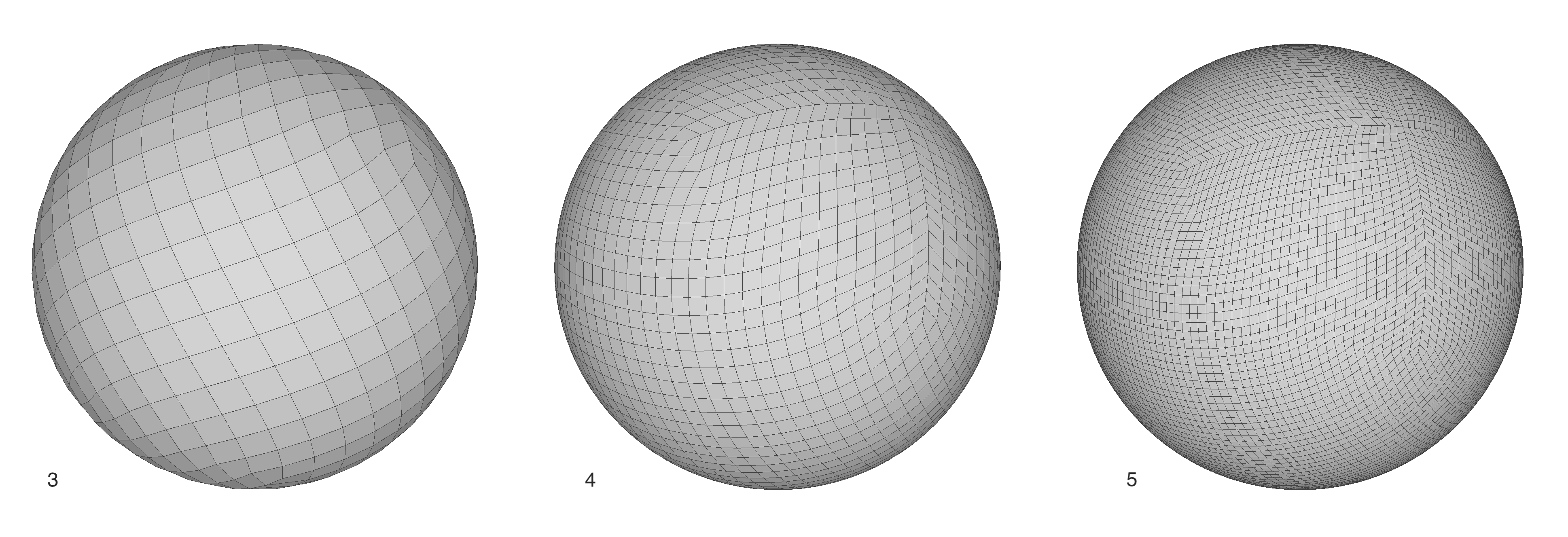
While there are many ways to partition the sphere, the HEALPix partition is notable for maintaining equal area cells and having a consistent, compact shape simultaneously (it is not possible to subdivide the sphere into cells that have equal area and equally spaced centers, so there is always a tradeoff). The former is essential for sampling (we don’t want to do on-the-fly corrections for varying solid angles), and the latter for appropriately localizing a cell on the sphere. While public source code for the official HEALPix partition is available from JPL, its (GPL) license is not compatible with DIRSIG and our implementation has be developed independently based on:

Roukema, B. F., & Lew, B. (2004). A Solution to the isolatitude, equi-area, hierarchical pixel-coordinate system. arXiv preprint astro-ph/0409533.

As such, indexing and alignment may vary between the DIRSIG5 implementation and the HEALPix library.

Our usage of the HEALPix partition takes advantage of the hierarchical nature of the subdivision, treating the representation as twelve quad-tree data structures (one quad-tree for each of the original twelve cells). This allows for quick traversal of the data (the maximum number of steps equal to the full depth) and we do an initial data compression based on comparison of child-nodes (i.e. approximately constant valued child cells can be collapsed into the parent and less data stored). Finally, we can use the diamond-shape structure itself as the basis for an interpolation scheme across the surface of the sphere to overcome quantization.

In order to provide the functionality described above (BRDF and DHR queries plus sampling), the structure of the SQT is as optimized as possible. First, we recognize that incorporating the projected area is essential for maximizing the contribution of each sample. So rather than store the BRDF directly, we store the cosine weighted BRDF for a given exitant angle.

Second, the primary role of the SQT is to provide a quick route to sampling the cosine weighted BRDF. We pre-normalize the hemisphere so we are left with the PDF of the DHR. This allows us to traverse the 12 quad-trees with a single random number draw from [0,1]. The scalar magnitude of the DHR is stored separately and can be recombined when querying the (cosine-weighted) BRDF.

This separation of the shape from the magnitude suggest our approach to handling spectral variation. Each SQT is only valid for a single wavelength (and a single source/view vector) and it would be very costly to rely on an independent SQT for every posssible wavelength in a simulation. Instead we recognize that in most instances, the "shape" (i.e. the PDF) of the reflectance function does not vary as quickly as the magnitude (i.e. the magnitude). Therefore, we can define the shape at a coarser spectral sampling rate than the magnitude and simply interpolate the shape between spectral samples. This allows us to bring in more finely sampled DHR data than we might have for full bidirectional data.

The "RAW" optical format is intended to hold sample optical property data for one or more exitant angles, a set of wavelength samples, and arbitrary scattered directions. Each set of optical property data is stored in a single file containing:

The raw data can be irregularly spaced across the hemisphere or sphere. The exitant angles and wavelength samples can’t change though and data must be provided for each spectral point.

The "SQT" optical format is intended to hold preprocessed optical property data that has been sorted into a Spherical Quad-Tree. Besides the human-readable header, it is exclusively machine generated, binary, may be compressed internally. It is used to quickly load optical property data into a simulation and should only be inspected with appropriate tools (though the header is human readable). It consists of: