This plugin was created to allow users to easily collect either the inbound spectral radiance onto a point or the outbound spectral radiance from a point.
Summary
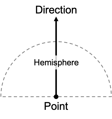
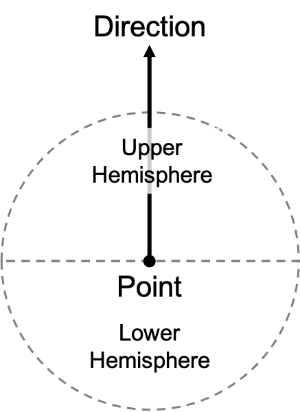
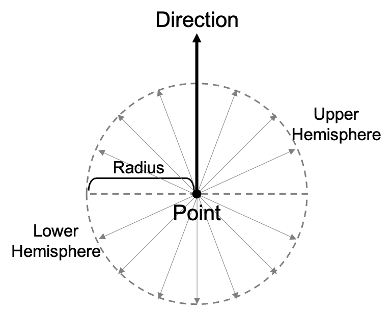
Hemisphere vs. Sphere Collection Coverage
The user can choose to measure either over a hemisphere or an entire
sphere around the point. The center of the sphere or hemisphere is defined
by a scene ENU point in space and then a direction vector that defines the
orientation or "up" direction. The default direction is the scene ENU "up"
direction (+Z or 0,0,1), but the user can change the orientation of the
coverage surface by specifying an alternative direction vector.
Orthographic vs. Polar Projection
The second component of the collection geometry is the projection scheme. The role of the projection scheme is to define how XY pixel locations in the output image are mapped to zenith and azimuth samples in the hemisphere or sphere.
Using hemispherical coverage as an example, the orthographic projection scheme writes the radiance values to the output image such that the azimuth samples are written in the X dimension and the zenith samples are written to the Y dimension. The user has control over the number of zenith samples (between 0 → 90 degrees) and azimuth samples (between 0 → 360 degrees).
|
|
With this projection scheme, the zenith and azimuth dimensions are sampled on constant intervals in the respective dimensions. |

|
|
If the coverage type is hemispherical, the output image is X x Y pixels. If the coverage type is spherical, the output image is X x (2Y) pixels (one XY grid for the upper hemisphere and a second XY grid for the lower hemisphere). |
The alternative option is the polar projection scheme. In this scheme, the XY dimensions of the image are used to define a polar coordinate system and the zenith and azimuth radiance samples are projected into the output image. The circular aspect of the polar projection is mapped into a square XY grid in the output image, so the number of X and Y samples is expected to be equal (or the larger of the two is used). The output radiance values are computed by computing the zenith and azimuth mapped to each location based on the polar projection. The X dimension of the output image effectively defines how many samples are used in the zenith dimension. Since this dimension spans 90 degrees declination for both 0 and 180 degrees azimuth, the effective zenith sampling interval is 90 / 2 / X = 45 / X degrees per sample.
|
|
Any pixels in the image grid that map to a zenith greater than 90 degrees (e.g. the corners of the image) are skipped. |
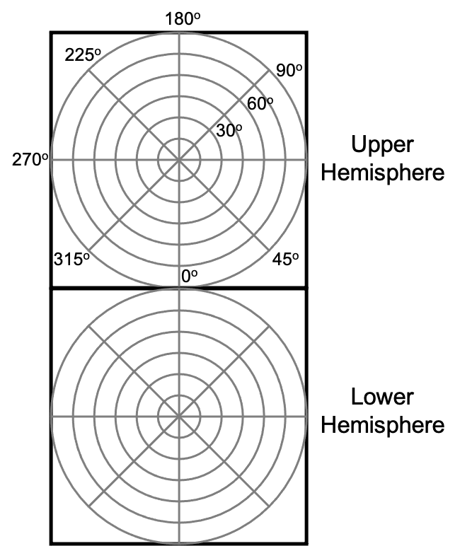
|
|
If the coverage type is hemispherical, the output image is X x Y pixels. If the coverage type is spherical, the output image is X x (2Y) pixels (one XY grid for the upper hemisphere and a second XY grid for the lower hemisphere). |
Inbound vs. Outbound Modes
The collector has two primary collection modes.
The inbound mode collects the spectral radiance arriving onto a point
in space. This collection mode is minimally defined by a point in space
and the direction (default is "up" or 0,0,1).
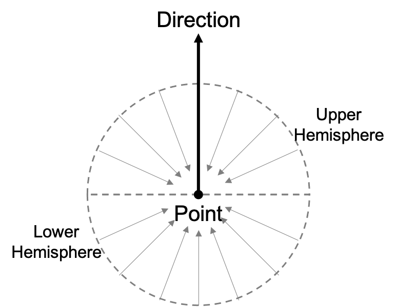
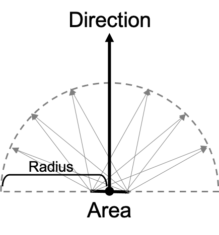
The outbound mode collects the spectral radiance leaving a point in
space. This collection mode is minimally defined by a point in space,
the direction (default is "up" or 0,0,1) and a radius. The radius is used to define at what distance
from the point the radiance is collected.
The outbound collection can also be used to collect radiance from a non-zero area. A pair of optional, axis-aligned X/Y width variables can be used to define a region around the target point that will be sampled by each location on the sphere or hemisphere.
Input
The input configuration file is a JSON formatted description. The file
has two main sections: input and output. An example is shown below:
{
    "input" : {
        "bandpass" : {
            "minimum" : 0.45,
            "maximum" : 0.7,
            "delta"   : 0.05
        },
        "date_time" : {
            "start"      : "2009-09-01T12:10:00.0000-05:00"
        },
        "location" : [0, 0, 5],
        "direction" : [0, 0, 1],
        "mode" : "inbound",
        "coverage" : "sphere",
        "projection" : "orthogonal",
        "xsamples" : 180,
        "ysamples" : 180
    },
    "output" : {
        "filename" : "inbound_ortho.img"
    }
}
Input Parameters
Spectral Bandpass
The primary output is a spectral radiance cube defined by a bandpass that has a spectral minimum, maximum and sampling delta (units are microns).
        "bandpass" : {
            "minimum" : 0.45,
            "maximum" : 0.7,
            "delta"   : 0.05
        }
Date/Time
The starting date/time for the collection is described in the
date_time section. The start variable is an ISO8601 date/time.
        "date_time" : {
            "start"      : "2009-09-01T12:10:00.0000-05:00"
        }
This plugin can also collect a series collections over time.
The number of temporal measurements is defined by the step_count
variable and the time between measurements (in seconds) is defined
by the step_time variable. The example below collects a series of
10 collections starting at 12:10 with each subsequent measurement
occurring on 1 hour (3600 seconds) intervals.
        "date_time" : {
            "start"      : "2009-09-01T12:10:00.0000-05:00",
            "step_count" : 10,
            "step_time"  : 3600.0
}|
|
It is considered an error if the step_count is greater than 1
and the step_time is not set or is not non-zero and positive.
|
Location
The location defines where in the scene the collection point is located
(in Scene ENU units).
Direction (optional)
The optional direction defines the direction to the top of the hemisphere
for a hemispherical and spherical coverage scenario. The default direction
is 0,0,1.
Direction Mode
The mode describes if the collection is measuring the inbound radiance
arriving onto the defined location ("mode" : "inbound") or the outbound
radiance leaving from the defined location ("mode" : "outbound").
-
In the case of an outbound scenario, the user must provide the
radiusdefining the distance from the defined location that the radiances are collected. -
In the case of an outbound scenario, the user can provide an optional rectangular area (via the
xwidthandywidthvariables) about the location that will be sampled.
Coverage
The coverage variable defines if the collection will sample either a
hemisphere ("coverage" : "hemisphere") or sphere ("coverage" : "sphere").
Projection and Samples
The projection defines how hemisphere or sphere is sampled and represented
in the output data cube file. The orthogonal projection directly couples the
output image X axis to the azimuth sampling dimension and the Y axis to the
zenith sampling dimension ("projection" : "orthogonal"). The polar
projection maps the zenith and azimuth into the X/Y axes of the output
image to produce circular or fisheye style visualizations.
The xsamples and ysamples define the number of samples in the zenith
and azimuth dimensions. In general, these two parameters define the
dimensions of the output image cube.
|
|
If a spherical coverage is requested, the image will be 2x larger in the Y dimension to account for the upper and lower hemisphere. |
The Output Parameters
Filename
The name of the output ENVI image file. This filename is split into a
basename and file extension. If the step_count is greater than 1, then
the output filename will include the capture or "step" index in it (e.g.
example_0.img, example_1.img, etc.).
|
|
This plugin honors the --output_folder and --output_prefix
command-line options.
|
Output
The output generated by this plugin is a spectral data cube with
two spatial (angular) dimensions and one spectral dimension. The
spatial (X/Y) dimensions are driven by the input xsamples and
ysamples variables. If a "coverage" is "spherical", the ysamples
will be repeated across the upper and lower hemisphere, doubling
the number of total samples in this dimension.
The units of the output spectral radiance image data cube are Watts/(cm2 sr micron).
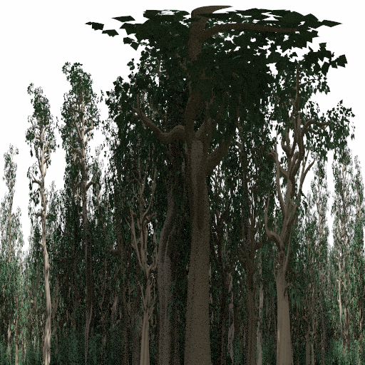
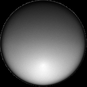
Orthographic Projection Example
The image below shows the output of an orthographic projection collection in a jungle scene. The apparent distortion at the top of the image reflects the solid angle of the samples getting smaller but being represented in the output image as a single pixel.
|
|
The orthographic projection is most useful when using the output as the input to another model because the zenith and azimuth indexing is straightforward. |
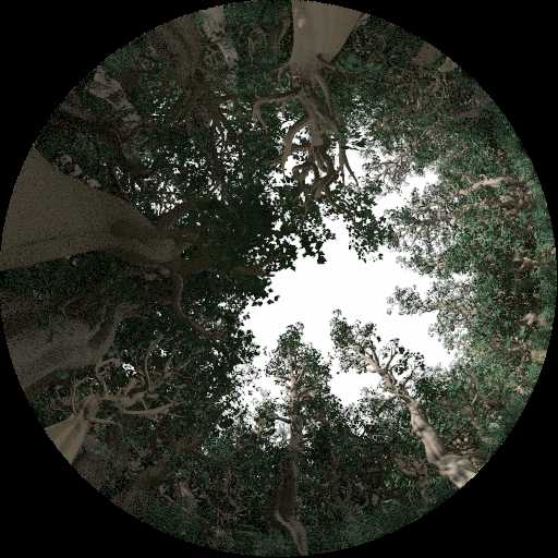
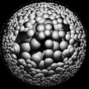
Polar Projection Example
The polar projection option produces traditional "fisheye" type
data, which can be more intuitive for visualization purposes. In
this case the xsamples and ysamples are used to define a square
grid into which the zenith and azimuth samples are projected. As
a result, the output image contains a circular border around the
projected samples (these border pixels have values of zero). The
outer ring of pixels correspond to a zenith (declination) angle of
90 degrees and then progressing to smaller and smaller zenith
(declination) angles toward the middle of the image.
|
|
The polar projection is most useful for visualizations of the environment around an object. |
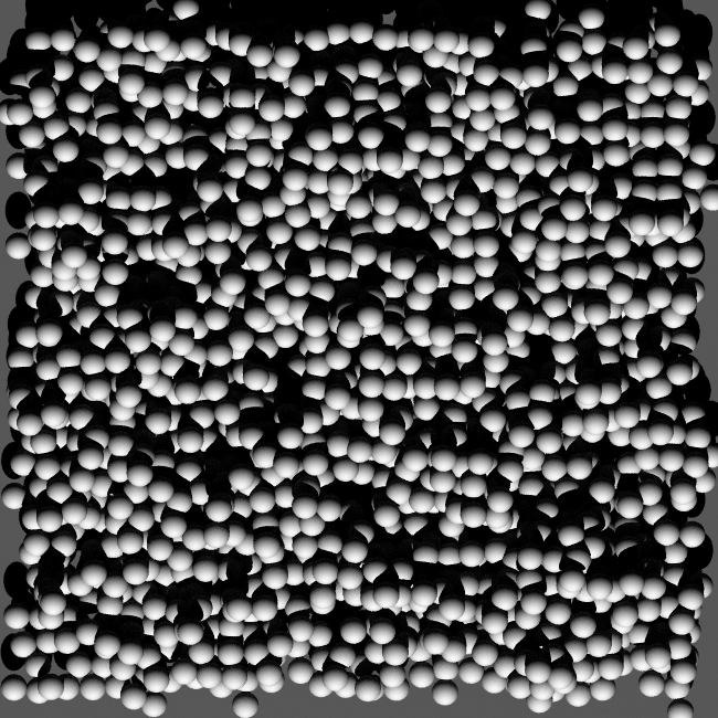
Outbound Area Sampling Example
The outbound collection mode can collect the radiance from either a point
(the location) or averaged over an area (centered on the location and
sampled over an area defined by the xwidth and ywidth).
The data provides a polar visualization of the radiance reflected by the scene into the hemisphere above the scene. The distribution shows that the radiance reflected by the scene is higher into the 180 degree azimuth direction, which corresponds to the -Y direction in the scene. This is the backscatter direction of the spheres
The GSD for this simulation is 30 meters, which encompasses the region covered by the spheres.
Usage
To use the SphericalCollector plugin in DIRSIG5, the user must use the newer
JSON formatted simulation input file (referred to a JSIM
file with a .jsim file extension). At this time, these files are
hand-crafted (no graphical editor is available).
The user has two choices for how to construct the input. The first option is to embed the JSON description for the collector in the JSIM file, which results in a self-contained simulation configuration. An example is shown below:
[{
    "scene_list" : [
        { "inputs" : "./demo.scene" }
    ],
    "plugin_list" : [
        {
            "name" : "BasicAtmosphere",
            "inputs" : {
                "atmosphere_filename" : "./demo.atm"
            }
        },
        {
            "name" : "SphericalCollector",
            "inputs" : {
                "input" : {
                    "bandpass" : {
                        "minimum" : 0.45,
                        "maximum" : 0.7,
                        "delta"   : 0.05
                    },
                    "date_time" : {
                        "start"      : "2009-09-01T12:10:00.0000-05:00"
                    },
                    "location" : [0, 0, 5],
                    "direction" : [0, 0, 1],
                    "mode" : "inbound",
                    "coverage" : "sphere",
                    "projection" : "orthogonal",
                    "xsamples" : 180,
                    "ysamples" : 180
                },
                "output" : {
                    "filename" : "inbound_ortho.img"
                }
            }
        }
    ]
}]
The second option is to place the JSON collector description in a separate file and supply the name of that file in the JSIM file:
[{
    "scene_list" : [
        { "inputs" : "./demo.scene" }
    ],
    "plugin_list" : [
        {
            "name" : "BasicAtmosphere",
            "inputs" : {
                "atmosphere_filename" : "./demo.atm"
            }
        },
        {
            "name" : "SphericalCollector",
            "inputs" : {
                "input_filename" : "./demo.json"
            }
        }
    ]
}]
Demos
The SphericalCollector1 and SphericalCollector2 demos contain a working examples of this plugin.