Overview
Numerical integration is a central component of a complex radiometric simulation tool. In order to accurately perform integrations of discrete functions in a reasonable amount of time, the function is usually sampled. Regular or uniform sampling of some discrete functions can give rise to artifacts including aliasing. In addition, uniform sampling can be inefficient because computing the contribution for each sample of the function can be costly and uniform sample doesn’t prioritize getting the contributions for the "most important" regions of the function.
Example
In order to illustrate the process for importance sampling a function, the following example function will be used:
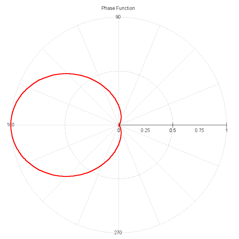
\begin{equation*} f( \theta ) = \cos^5 \left ( \frac{|180 - \theta|}{2} \right ) \end{equation*}
This function approximates a "scattering phase function", which is a function that describes the probability of an incident photon interacting with a particle (or molecule) and scattering in a new direction. The magnitude of the function as a function of angle describes the directional probability. The plot below shows the example phase function plotted in polar coordinates. The magnitude of the function is significantly higher in the forward scattering direction (angles near 180 degrees).
In the context of a ray tracer, an efficient way to compute the new scattering direction for a photon is sought. As the function illustrates, a photon should be scattered in the forward directions with a significantly higher probability. Therefore, we want to method to use this function to drive a semi-random mechanism that will compute new photon directions (angles) such that the ensemble direction statistics are correct. If a large number of new directions are pulled from this mechanism, the normalized histogram of the directions should reproduce the input function.
Probability Functions
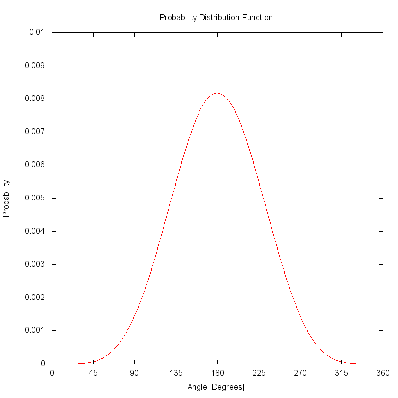
The plot below illustrates the same phase function as a 1D Cartesian function. The function has been area normalized to produce a probability distribution function (PDF).
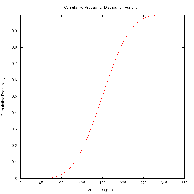
The cumulative distribution function (CDF) is created by accumulating the PDF function. If the PDF was correctly area normalized, the CDF will eventually reach a peak value of 1.
Look-up Table
The key component in an importance sampling scheme is the function that will reproject an otherwise uniform distribution of random samples. This function is usually implemented as either an analytical function (when one can be derived) or as a look-up table.
For this example, a look-up table (LUT) approach is used where a uniformly disributed random input values between 0 → 1 can be directly indexed into a finite array of output values. To create the LUT to map input to output values, the input angles for the CDF were range normalized and then the CDF was transposed. The plot below shows the look-up table (LUT) created from the CDF.
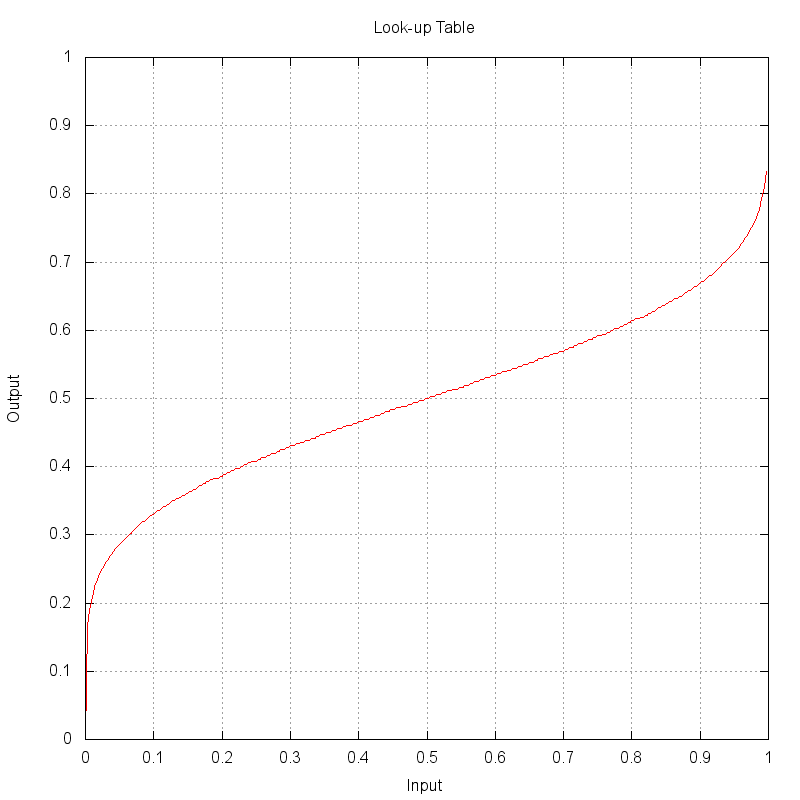
A diagonal line (slope = 1) would produce a null projection. In
this example, it can be seen that an input value of 0.2 results
in an output value of nearly 0.4. The shape of this LUT projects
the smaller (nearer 0) and larger (nearer 1) values closer to 0.5.
This projection will end up remapping uniformly distributed points
closer to the central value of 0.5, which is what is desired to get
more samples closer to the center lobe of the input PDF.
Uniform vs. Importance Samples
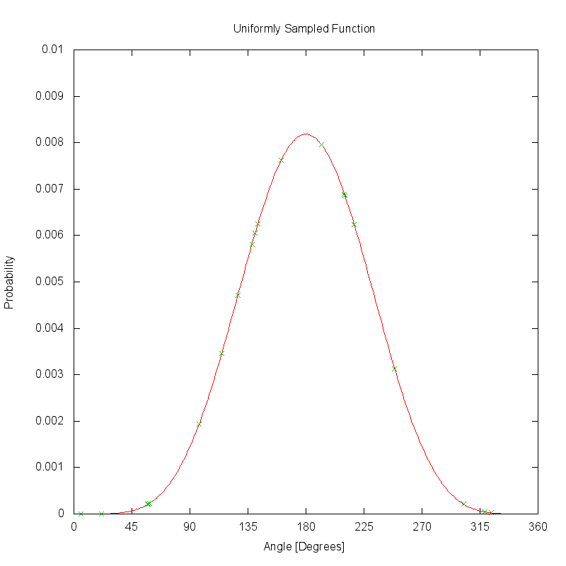
The plot below shows how the PDF would be sampled with 20 uniformly distributed samples. The green points on the curve show the locations of the 20 samples, which uniformly sample the regions of the function with low magnitude as well as those regions where the magnitude is much higher.
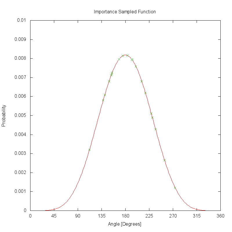
The plot below shows how the same PDF would be sampled if the same 20 uniformly distributed samples are reprojected by the look-up table (LUT). Unlike the uniform sampling scheme, these samples are clustered near the highest magnitude regions of the PDF.
Summary
Although the concept of importance sampling was illustrated here for a 1D function, these same techniques can be applied to multi-dimensional functions. The challange in developing importance sampling schemes is creating an efficient redistribution mechanism.
The DIRSIG model using importance sampling in the following areas:
-
Sampling (1D) scattering phase functions
-
Sampling (2D) bi-directional reflectance distribution functions (BRDFs).