A height model (<heightmodel>) is a sub-declaration of the height field geometry object. Whereas the height field generically describes a geometric surface based on regularly sampled set of heights, the height model describes the specific height driver underlying that data.
As mentioned in the height field entry, the purpose of these tools is to allow a convenient mechanism for building geometry directly from static height data (e.g. terrain) and to provide a mechanism to support dynamic height fields (e.g. water waves) that would otherwise be too difficult or impossible to model with existing geometry inputs.
The models described below are divided into static and dynamic categories, where dynamic height fields may change over time and static ones are constant. When using dynamic height fields, a set of recently used data is held in memory as a function of time (to facilitate non-sequential queries, such as per-pixel integration). The default cache size (set in the <heightfield> entry) is fairly large, but can be modified if needed (see the ‘<cachesize>’ option to the height field). Note that unused cache data does not take up memory or diminish run time, so its fairly safe to leave it at the default value unless you know you’ll need more (e.g. you sample the exposure time a number of times greater than the default) or want to minimize memory usage.
Introduction
The height models share two basic components. First, they are wrapped by the <heightmodel> tag. Second, the <heightmodel> tag takes a single attribute, "type" which indicates which model should be parsed and loaded. The full entry will look something like this:
<object>

  <basegeometry>
    <heightfield>
      <matid>100</matid>
      <heightmodel type="wave">
        ...
      </heightmodel>
    </heightfield>
  </basegeometry>

  <staticinstance/>

</object>
where the entries within the height model are specific to the type.
Height model types
Wave height model (type="wave")
The wave height model provides a mechanism to generate a wind-driven wave surface in DIRSIG based on a wave frequency spectrum (<spectrum>). The approach take in DIRSIG is based on the work of Mastin et al ("Fourier Synthesis of Ocean Scenes" (1987)). The wave frequency spectrum is usually based on point samples of wave heights (e.g. buoy measurements) and represents waves traveling in all possible directions. Therefore it is necessary to define a spreading function that describes how that spectrum is distributed angularly (<spread>). Finally, we also need to drive the wind speed as measured from a particular height (10m above sea level) which has its own model (<wind>). Note that this wind speed is currently independent from any other wind speeds in DIRSIG (e.g. as defined in the weather file).
After constructing a fully directional frequency spectrum of the wave surface, it is used to filter the Fourier transform of a random surface. Once we return from frequency space, we’re left with a surface that is representative of the frequencies in the model. Additionally, by carefully manipulating the phase of each wave (based on wave dispersion relations since they travel at different speeds), we can animate the surface as a function of time. A typical wave model definition might look like:
<heightmodel type="wave">
  <spectrum type="JONSWAP">
    <gamma>3.3</gamma>
    <fetch>1e6</fetch>
  </spectrum>
  <spread type="COS2S">
    <s>8</s>
  </spread>
  <wind type="CONSTWIND">
    <speed10>6</speed10>
    <direction>-90</direction>
  </wind>
  <nelements>1024</nelements>
  <width>40</width>
</heightmodel>
All wave height models are currently described for a square area (to simplify some of the internal calculations) with the side of the square defined by <width> in meters (though the height field can be non-uniformly scaled via the instance transform). The number of actual elements used (i.e. the number of height sample points) is driven by the <nelements> entry which gives the number of samples along one dimension. The number of sample points dictates the resolution of the height field and is usually selected such that the facetization is sub-pixel (in this case the longest edge of a triangle would be 40/1024 = 4cm).
Wave spectra
-
PM(Pierson and Moskowitz 1964)-
this is a classic first generation wave model that assumes a fully developed sea state and does not represent non-linear wave-to-wave interactions
-
no parameters are supplied to this model (except for the wind speed generated by the wind component)
-
-
JONSWAP(JOint North Sea WAve observation Project — Hasselmann et al. 1973)-
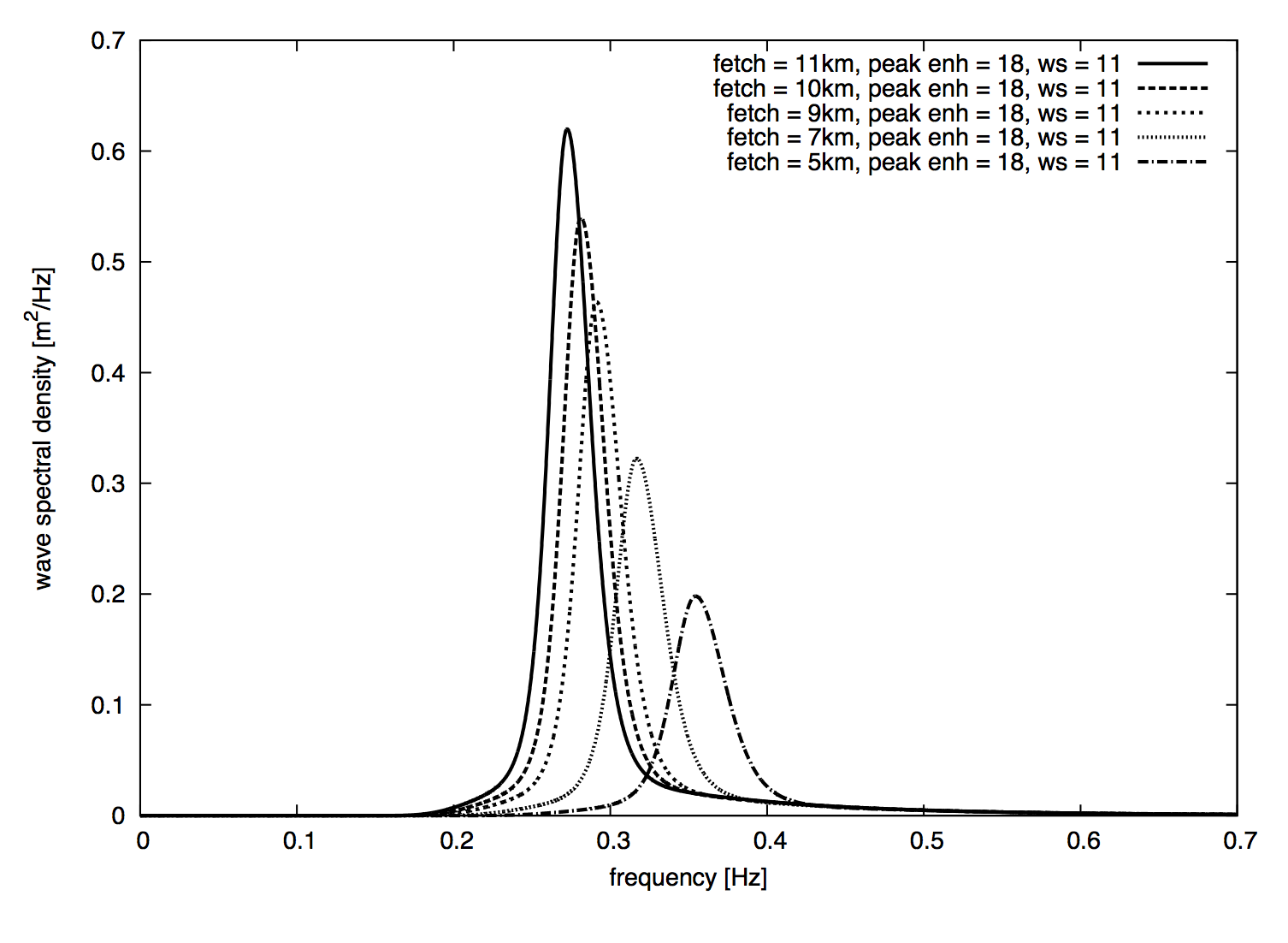
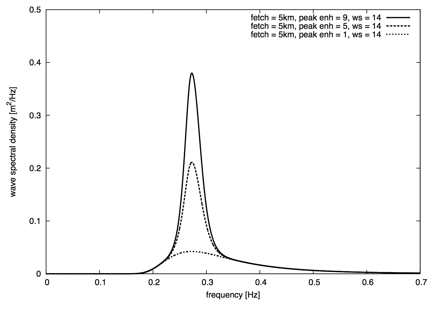
this spectrum is popular correction to the Pierson-Moskowitz spectrum that incorporates non-linear effects via a peak-enhancement factor and the fetch length (distance along which the wind has blown at a constant rate)
-
the JONSWAP spectrum is parametrized by the
fetchlength (in meters, though it is usually on the order of km) and the base of the peak enhancement factorgamma -
the effect of varying the two JONSWAP spectra parameters is shown below (note that a gamma value of one results in a Pierson-Moskowitz spectrum)
-
Spreading functions
-
COS2S(cosine of the angle from the wind vector to a power)-
this is a simple power of the cosine of the angle parametrized by an integer value
<s>such that the spread is calculated as cos^2s
-
Wind speed
-
CONSTWIND(constant wind speed and direction)-
sets the windspeed
<speed10>in m/s measured at 10 m above the water surface -
sets the wind
<direction>(source of the wind measured in degrees clockwise from North) -
conversion from a wind speed measured at 19.5m above the surface (another common value) to 10m above the surface can be done by multiplying by roughly 0.975
-
note that this wind model is for the wave surface generation only and won’t be used elsewhere in the simulation
-