Optical Property Modeling Handbook

This document discusses an approach to using the DIRSIG image and data generation model to generate BRDF/BRF or other optical property models from scene geometry and materials. The manual is based on work done to replicate the RAMI (RAdiation Model Intercomparision) results and comparisons with that data will be presented as examples.

Overview

The DIRSIG model is designed to support end-to-end sensor modeling rather than the specific types of radiometry setups needed to build models of optical properties. However, the underlying radiometry engine is certainly capable of doing this type of study and with a few special tools, generation of these types of models can be fairly straightforward.

While there are no particular limitations to the type of simulated optical property model that can be generated in DIRSIG, we are usually motivated by a desire to describe geometrically and optically complex phenomena in a compact form. For example, the return from a tree canopy as seen by a satellite with a >10m GSD sensor could be modeled directly in DIRSIG by modeling each tree in the canopy with every leaf and every branch having geometric and optical property models. However, a very large number of detector rays are necessary in order to capture the geometric complexity within each pixel — and all that fine detail is lost once integrated over the solid angle of the detector. A much more effective way to model the signal from the canopy might be to understand the aggregate reflectance off the top of the canopy that is a result of all the complex scattering from leaves and branches and to describe that in a simple parametrized reflectance model (that would probably vary over a horizontal area).

The goal of this document is to describe how to use DIRSIG to generate the simplified representation of a complex process by generating very compact and controlled experiments. In the case of modeling a tree canopy, we would generate small, representative sections of the entire canopy and use them to build up an understanding of the effective reflectance.

Technical Readiness

This application area is currently ranked as operational. While the fundamental radiometry engines underlying the approach are mature, some of the tools used to facilitate efficient generation of optical models are still fairly experimental. The operational status also means that a lot of techniques and tools used in this manual are not available from within the GUI and requires hand editing of some of the input files. Some familiarity of what files go into a DIRSIG simulation and their general structure is assumed

Theoretical Background

The remainder of the manual will be focused on generating reflectance models using DIRSIG. However, the same general approach applies to generating transmittance or general scattering optical properties.

The specific type of reflectance model that we want to generate is a BRDF, or a Bidirectional Reflectance Distribution Function, which describes the radiance at a given wavelength scattered from a surface into a particular direction given the irradiance onto that surface from another direction. In other words,

\( \mathrm{BRDF}(\theta_r, \phi_r, \theta_i, \phi_i, \lambda) = \frac{dL_r(\theta_r, \phi_r, \lambda)}{L_i(\theta_i, \phi_i, \lambda)\cos{(\theta_i)}d\omega_i} \),

where the incident radiance has a corresponding differential solid angle. If we integrate over the entire hemisphere above a surface then we get the total reflected radiance,

\( L_r(\theta_r, \phi_r, \lambda)=\int_{\Omega_i}\mbox{BRDF}(\theta_r, \phi_r, \theta_i, \phi_i, \lambda){L_i(\theta_i, \phi_i, \lambda)\cos{(\theta_i)}d\omega_i} \),

which is usually the desired usage (and the type of optical property needed by DIRSIG). Therefore, in order to build a model of reflectance, we need to find the value of the BRDF for a set of incident angles, a set of exitant angles, and a range of wavelengths. That said, many materials can be described by simply knowing the azimuth angle between the incident and exitant directions, rather than the absolute angles (i.e. there is no dependence on the orientation of the material itself). Once we have the necessary values we can either use them directly (i.e. a data based model) or to find a good fit with another model or multiple models.

Another form of the BRDF is a BRF (Bidirectional Reflectance Factor), which is simply the BRDF relative to a 100% reflecting Lambertian surface, i.e.

\( \mbox{BRF}=\pi \cdot \mbox{BRDF} \)

While not directly useful in DIRSIG, the BRF is the form used by the RAMI participants and plots in this manual will be of the BRF values rather than BRDF values.

Because of the potential computational complexity and memory requirements of the methods used, we will restrict our optical property generation to a single wavelength at a time (this is not a requirement, but the inputs for a spectral calculations would be more complex). It is suggested that the initial setup should be focused at calculating a single wavelength and then once confident with the output from that simulation, additional wavelengths can be run independently or the inputs modified to run all wavelengths simultaneously.

Spectral considerations

DIRSIG is normally run by computing all spectral samples simultaneously, often doing calculations on 100s or 1000s of wavelengths at once. Under normal conditions, it is straightforward to account for spectral differences at surfaces (they are primarily differences in magnitude) if we ignore things like spectral dispersion in the atmosphere.

Modeling of a tree canopy, however, requires modeling tens or hundreds of scattering events along paths between the detector and the source, which compounds small spectral differences in the transmittance and reflectance. Therefore, some of the methods used allow photons to follow different potential paths based on their wavelength. For visible region radiometry the potential path variations are limited (photons are only multiple scattered a handful of times on average). In those cases the computational complexity is low and more wavelengths can be calculated simultaneously.

On the other hand, radiometry in the near infrared (common for canopy simulations) is dependent on higher orders of scattering since the probability of either reflecting off of, or being transmitted through, a leaf is usually very high. For these types of scenarios we need to model a large population of possible paths that photons will take and it is often easier to run a single, or a just a few, wavelengths at a time.

Components of the Simulation

The simulation used to generate the reflectance model consists of three major components:

A single source providing the irradiance onto the surface
A constrained scene modeling the underlying structure of the BRDF
A single (sub-sampled) detector collecting the reflected radiance

By varying the angle of the source and detector relative to the scene, we are able to generate a full representation of the BRDF.

Setting up a Simulation

For the purposes of this manual, it is assumed that the user has a basic understanding of how to setup a simulation in DIRSIG. Given that, we will focus on the three components listed above and describe how to set them up in detail.

Modeling the Source in DIRSIG

While there are a number of source types available in DIRSIG, the most straightforward way of defining the incident irradiance onto our scene is by using using one of the simplified atmospheric models available. Using an atmosphere is easy to setup and it also inherently assumes that the primary source (the sun) is far enough away that the angle does not change over the extent of the scene (which means that the incident angles will be constant over the scene as desired for the BRDF model).

In particular, we can use the "uniform" atmospheric model which divides the atmosphere into two components: a uniform hemisphere and a sun-sized source. This atmosphere model takes a single irradiance value which is split between the irradiance coming from the hemisphere as measured by a flat plate in the local coordinate system of the scene, and the "scalar" irradiance of the sun. The scalar irradiance is the irradiance that would be measured on a surface perpendicular to the directional vector of the source; that means that the irradiance onto the same scene flat plane would be the scalar irradiance weighted by the cosine of the sun zenith angle to account for the projected area differences.

For the BRDF model we want the hemisphere irradiance to be zero since we only want to know the amount of radiance scattered from a single direction. Furthermore, the scalar irradiance, E', of the sun in our simplified model is equivalent to the (average) radiance of the sun integrated over its solid angle. With this in mind, we can rewrite our earlier equation for the BRDF as:

\( \mbox{BRDF}(\theta_r, \phi_r, \theta_i, \phi_i, \lambda) = \frac{dL_r(\theta_r, \phi_r, \lambda)}{E'_i(\theta_i, \phi_i, \lambda)\cos{(\theta_i)}}, \)

and

\( \mbox{BRF}(\theta_r, \phi_r, \theta_i, \phi_i, \lambda) = \pi \frac{dL_r(\theta_r, \phi_r, \lambda)}{E'_i(\theta_i, \phi_i, \lambda)\cos{(\theta_i)}}, \)

By setting a convenient scalar irradiance,

\( E'_i=\frac{\pi}{\cos{(\theta_i)}},\)

our equation becomes

\( \mbox{BRF}(\theta_r, \phi_r, \theta_i, \phi_i, \lambda) = dL_r(\theta_r, \phi_r, \lambda),\)

and calculating the BRF is as simple as finding the reflected radiance reaching our detector for the exact set of view angles (and averaged over the horizontal extents the scene).

An atmosphere setup (the .atm file) for a source zenith angle of 20 degrees would therefore look like:

<atmosphericconditions>
  <metadata/>
  <uniformweather>
    <classicdata>
      <filename>$DIRSIG_HOME/lib/data/weather/mls.wth</filename>
    </classicdata>
  </uniformweather>
  <turbulence model="kolmogorov" enabled="1">
    <cn2 model="hv57">
      <windspeed>10</windspeed>
      <ground>1.7e-14</ground>
    </cn2>
  </turbulence>
  <ephemeris>
    <fixed>
      <solarazimuth>0.0</solarazimuth>
      <solarzenith>0.349066</solarzenith>
    </fixed>
  </ephemeris>
  <uniformradiativetransfer>
    <hemisphereirradiance>3.3432</hemisphereirradiance>
    <skyfraction>0</skyfraction>
  </uniformradiativetransfer>
</atmosphericconditions>

where the uniform atmosphere is setup in the last section and the total hemisphere irradiance (3.342 = Pi / cos(20) ) is allocated to the sun’s scalar irradiance.

The other important component of the atmosphere file is the fixed ephemeris of the "sun" location, as defined by a zenith angle (in radians) and an azimuthal angle (also in radians and measured clockwise from North). In the above example, the sun is placed at 20 degrees.

The downside of using the fixed ephemeris tool in the atmosphere model is that it will fix the sun position for the entire simulation. This may not be desired if we want to model multiple source angles in a single simulation. In that case, there is a "scripted" ephemeris model that allows the user to dictate the position of the sun as the scene progresses through a provided ECMA script (though the varying position means that the cosine factor will have to applied manually). Details on the scripted ephemeris model will be available soon.

Modeling the Scene in DIRSIG

Since our goal is to build a model of the effective BRDF of the scene, we can constrain the scene as much as possible so that its area is a match to the desired scale being modeled by the BRDF (note that if we want to model the variation in a BRDF in a single scene then the area would need to be larger than the desired scale in order to provide different windows to capture). To simplify and optimize the setup of the radiometry solvers used to handle multiple-scattering in the scene, we want to make the scene rectangular in outline and aligned with the X and Y axes of the local scene coordinate system. It is also convenient to place the center of the scene at the origin of the coordinate system.

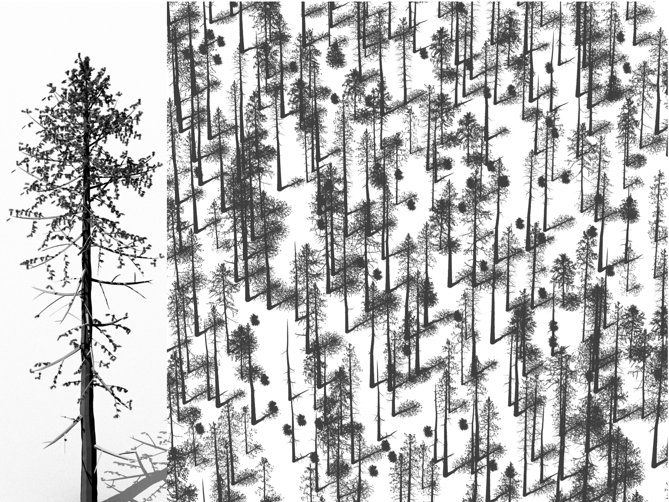
With these few considerations in mind, the contents of the actual scene are setup the same as any other scene in DIRSIG. For a canopy based scene we need both the terrain and the trees as modeled geometry that are attributed with appropriate optical properties. The RAMI experiments have good examples of complex geometric structure and limited spectral optical properties:

Figure 1. The RAMI Real Zoom-In geometry as rendered in DIRSIG. Leaves are modeled abstractly as scattering disks in discrete, shaped distributions (cylinders and spheres).

Figure 2. The RAMI Ofenpass pine stand geometry as rendered in DIRSIG. The Ofenpass trees are modeled down to individual pine needles and are rather sparsely distributed over flat terrain.

Leaves, bark, grass, etc… are most definitely not individually Lambertian reflectors/transmitters and yet that is often how they are modeled (in the RAMI scenes, for example). While certainly a simplification, this approach makes sense since we see these scene elements in aggregate and in random distributions of orientations (particularly leaves). That said, if more detailed BRDF/BTDF models are available, they can be used (one might expect the glossy reflection of some leaves to be particularly important for some species).

Modeling the Ground

The ground is a fundamental component of any scene. In addition to providing key scattering elements (grass, dirt, rocks, underbrush, etc..) it also provides a backstop for rays and photons entering the scene. Because of this its important to provide some sort of ground geometry (even if its just a plane).

DIRSIG does not automatically provide any base geometry for the earth. If a ray does not intersect any geometry in the scene being modeled then it will "pass through" the space that that Earth would occupy and end up passing through the atmosphere on the other side.

The recommended radiometry solver for the ground is the "Generic" rad solver in order to capture potential multiple scattered diffuse contributions. For example:

RAD_SOLVER_NAME = Generic
RAD_SOLVER {
    INITIAL_SAMPLE_COUNT = 1
    SAMPLE_DECAY_RATE    = 1
    MAX_BOUNCES          = 4
    MU_SAMPLES           = 8
    PHI_SAMPLES          = 10
    MIN_QUAD_SAMPLES     = 1
    PERMIT_DIRECT_ONLY   = FALSE
}

where the PERMIT_DIRECT_ONLY flag is explicitly set to false to elminate "quick" samples of the hemisphere above the surface (i.e. its important to make sure to capture the photons scattered off of the objects above the ground). Note that unless the ground terrain has a lot of variation we don’t need to worry about the computational complexity of the type of hierarchical ray tracing that the generic solver performs — rays traced from the ground surface will likely see the canopy (which truncates at the specialized multiple-scattering models described below) or the sky. A handful of bounces is a good maximum to use here to account for cases where we might go from ground to trunk to ground again (or similar).

The last consideration for the ground is to decide if the BRDF(s) being modeled should take into account the slop of the underlying terrain. A canopy BRDF modeled for a planar ground surface will not be valid for a forest canopy on the side of a hill (trees don’t grow perpendicularly to the ground plane so we can’t simply rotate the BRDF).

Modeling the Primary Scatterer Optical Properties

Background

The primary scatterers in a canopy scene will be the leaves or needles on the trees that both reflect and transmit photons incident upon them (in the near infrared in particular, both the reflectance and transmittance can be very high). The order of scattering due to these objects can be high (i.e. a photon can be reflected/transmitted tens or hundreds of times before leaving the canopy or being absorbed). If we were to try to capture this type of behaviour using the hierarchical ray-tracing radiometry tools in DIRSIG, we’d end up being faced with an exponential growth problem — to capture each successive order of scattering, we’d have to send out many new rays from each surface, which in turn would generate many more rays, etc…

The solution to this is to use one of the radiometry solvers in DIRSIG that are geared towards efficiently solving multiple scattering problems. A surface photon map based approach is well suited for capturing multiple scattering. It works by first doing a Monte Carlo propagation of photon bundles from sources into the scene, building an abstracted map of the flux density across surfaces and then using that map in a second pass to approximate the local multiple-scattered contributions.

The limitation of the photon mapping approach, however, is that we need to assume that the local area around where we are generating the multiple scattering contribution is uniform, in the sense that the local flux density is fairly constant. Simultaneously, we also need to make sure that the area from which we are making our estimate from the map is fairly large — large enough to collect a significant number of photon bundles to drive down noise. We can almost always satisfy both requirements by simply increasing the number of photons in the map to the point where the local population of photon bundles is high enough to get a good statistical distribution while keeping the area they are coming from small.

While photon mapping can be very successful for certain types of high multiple-scattering simulations, the problem with using that approach for tree modeling is that the map will be very sparse (corresponding to the surfaces of individual, independent leaves/needles) and our search areas will always have to be very, very small (the leaves/needles are themselves small and they also have edges which, if overlapped by the search area, drastically change the local density estimate). Increasing the number of photon bundles in the map only works up to a point since we start to run out of memory by the time we reach the fidelity needed.

To overcome these limitations we can use another, specialized radiometry solver called the goemetry density solver (GeoDensity). It functions just like the photon map, but instead of storing and searching an abstract structure, we associate photon bundles with geometry components (facets/primitives). This allows us to know the exact area onto which the photon bundles had the opportunity to fall allowing us to generate a very good approximation of the flux density. We also don’t have to worry about the edges of leaves/needles since the area is completely contained by the object surface (see figure below)

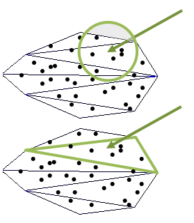
Figure 3. Comparison of local flux density estimation on a leaf using the photon mapping (top) and geometry density (bottom) radiometry solvers. Notional photon bundles stored in each solver are shown as black dots.

The limitations associated with the geodensity solver are even more severe than the photon mapping solver — we have lost all flexibility and are coupled to the fidelity of the underlying geometry (i.e. there is a single flux density estimate per facet, nothing more). To compensate for this we have to make sure that the geometry elements are fairly small and uniform — luckily, that is exactly what leaf geometry models usually are.

Assuming that the geometry is ready to be placed in the scene and has been attributed with materials, the geodensity solver can be setup as:

RAD_SOLVER_NAME = GeoDensity
RAD_SOLVER {
    MAX_BOUNCES = 100
    LOWER_EXTENT = -135, -135, -15
    UPPER_EXTENT =  135,  135, 0
    PADDING = 0
    TOP_ONLY = TRUE
    CYCLIC_BOUNDARY = TRUE
    DIRECT_ONLY = FALSE
    DISABLE_DIRECT = FALSE
    SOURCE_BUNDLES = 5e7
    SAVE_FILENAME = geoCyl5e7b100.sav
    LOAD_FILENAME = geoCyl5e7b100.sav
}

with parameters (and comments):

`MAX_BOUNCES`	The maximum number of scattering events to allow in the forward propagation of photon bundles from the source(s) :: For BRDF modeling this should be set high enough to allow the majority of photon bundles to scatter to extinction; a value of 100 should cover most canopy cases, including high scattering, near infrared simulations
`LOWER_EXTENT`	Minimum coordinate values [x,y,z] of a bounding box in scene coordinates encompassing the volume in which photon bundles should be shot into and stored
`UPPER_EXTENT`	Maximum coordinate values
`PADDING`	Fractional amount of the bounding box to extend the volume into which photon bundles are shot
`TOP_ONLY`	Only propagate photon bundles through the top of the bounding box; normally the projected area perpendicular to each source is used
`CYCLIC_BOUNDARY`	Propagate photon bundles that exit the bounding box to the opposite side of the box, allowing them to continue into the original :: Correctly setting up the bounding box is dependent on how the boundary conditions are handled — see discussion below
`DIRECT_ONLY`	Skip multiple scattering computations and only compute direct reflectance and transmittance from primary sources :: This is a useful flag to turn on to test the direct calculation portion of the radiometry solver (the flux density estimation is only used once bundles have scattered at least once, since direct ray tracing is more efficient before that)
`DISABLE_DIRECT`	Skip direct calculations and only include direct reflectane and transmittance from primary sources :: This is another flag that can be used to isolate the multiple scattering portion of the calculation for testing; note that setting DIRECT_ONLY and DISABLE_DIRECT will skip all geodensity calculations
`SOURCE_BUNDLES`	The number of photon bundles to propagate into the bounding box; there is no guarantee on the number of bundles that will actually be stored :: The number of source bundles drives the primary tradeoff runtime and fidelity; the more source bundles you have the better the solution will be, but the longer it will take to calculate (its usually a good idea to start with a lower value and increase by orders of magnitude until the simulation converges to an answer)
`SAVE_FILENAME`	Saves the stored photon bundles to the given file; since the association of bundles with geometry is based on a counter id, the scene must remain unchanged in order to load the file back in; note that if LOAD_FILENAME is present and set to the same file and the file exists, saving will be skipped :: This is a very useful feature once you start using many photon bundles to model the multiple scattering (and have a long propagation runtime). The save file will remain valid as long as the scene doesn’t change, so its possible to use the file while experimenting with sensor placement and collection scenarios.
`LOAD_FILENAME`	Loads a file that was previously saved; note that the file is a very simplistic serialization of the minimal data required to recreate the photon bundle storage — it should not be transferred between scenes or used with even a slightly modified version of the scene geometry that created it :: Its useful to set both the SAVE_FILENAME and LOAD_FILENAME as options (with the same argument — if the save file exists it will be loaded, if not, it will be created. The save file can also be used to isolate the multiple scattering portion of the return — by turning off the direct calculation and any other direct reflectance in the scene.

Scene Layout

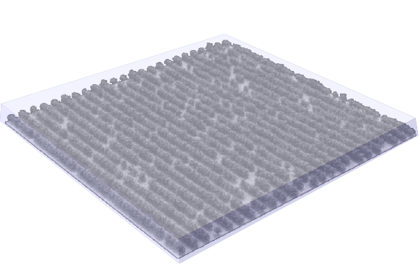
As suggested by the bounding box used to define the volume into which the geodensity photon bundles are shot, it is convenient to think about the scene (at least the part being used to generate the reflectance model) as being fully contained within a bounding box. That area may be the entire scene (see boundary conditions below) or it may be a portion of a larger scene. In general, its a good idea to only include the minimal amount of interacting geometry within a scene — anything not seen by the sensor directly or via scattering will just be wasted effort and load time. An example of a BRDF scene is shown below, where the entire RAMI Orchard scene is contained within a roughly 100x100x5m box.

Figure 4. The RAMI Orchard scene

Our goal again is to measure a single, average radiance coming from our scene over an area relevant to the scale we are trying to model. If the BRDF we are generating is meant to represent the entire bounded scene, then we can go ahead and use it directly. If not, and the desired scale is smaller, the smaller representation can be found by only viewing a portion of the scene at a time.

Averaging together smaller views of the scene is generally equivalent to just modeling the full scene, so there is no added benefit to viewing a scene multiple times unless the variation in the modeled optical property can be used (as a texture for instance).

If the desired area to be modeled is larger than the practical size limit of the scene (for instance, if a larger scene would require more memory than is available) then a representative optical property for a larger are can be made by averaging together solutions from variants on the scene (by rotating the scene or, preferably, introducing another random arrangement of geometry).

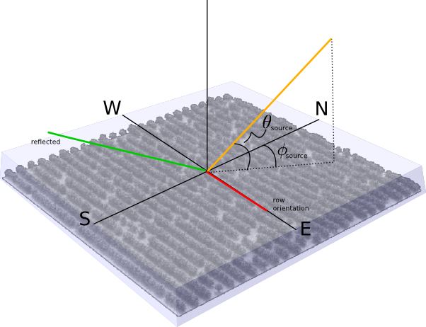
Once we have the bounding volume, we then need to setup the local coordinate system for the resultant BRDF. As we saw earlier, placement of the source and detector can be arbitrary — what matters are the angles relative to each other and relative to the orientation (if any) of the scene. Most of the time, orientation of the scene will not matter (i.e. if there is approximate rotational isotropy). For others though, there will be an inherent anisotropy (such as the "rows" in the Orchard scene). Modeling the former only needs to look at the relative angles between the source and view, while the latter requires the full set of angles to be modeled. The local coordinate system can be chosen for convenience, such as aligning the x-axis (East in the DIRSIG local coordinate system) with the orientation of the rows:

Figure 5. The RAMI Orchard scene with local coordinate system

Once the orientation and horizontal extents are chosen, we can add an additional convenience of placing the origin of the cooridnate system at the top of the bounding box encompassing the scene (i.e. the reference plane being sampled to find the reflected radiance). Doing so means that angles relative the the reference plane always match natural angles in the coordinate system — simplifying the setup of the source and detector.

DIRSIG’s Local Coordinate System

Every scene in DIRSIG has a local, right-hand-rule, cartesian coordinate system whose origin is tied to a specific geodetic point (as set in the .scene file). This space is based on a plane tangential to the surface of the earth (where the altitude of the surface relative to the WGS84 ellipsoid is part of the origin definition). Axes are oriented such that the x-axis points towards East and the y-axis points North (the so-called ENU [East, North, Up] orientation).

The XYZ to ENU mapping is not a standard and other mappings are often used. For example, the RAMI scenes are defined using an XYZ to NWU [North, West, Up] mapping (i.e. it is rotated 90 degrees from the DIRSIG system).

Boundary Conditions

Background

Once we have settled upon the bounds of the scene being modeled and the coordinate system in use, we still need to consider what happens when we reach the edges of the boundary. If the area being modeled (i.e. where the radiance is being measured) is smaller than the bounds then it can probably be used as is. If not, we need to handle the following:

Scattering from outside the bounds: We need to consider the fact that there are photons that would interact with the surrounding area and then enter/re-enter the bounded region, contributing to the total scattered signal.
Direct radiance from outside the boundary: When viewing the scene from any angle off-nadir there is the possibility of seeing through the existing scene.

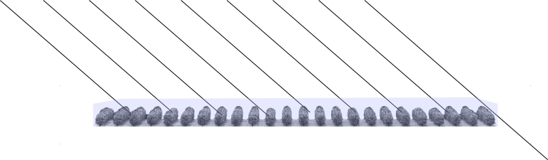
The second is easiest to visualize — if we cover the same area as a nadir view that covers the entire scene, then a slant view will always see directly outside of the bounds as long as there are any gaps in the scene:

Figure 6. The RAMI Orchard scene being viewed at a slant; rays entering the farther end of the scene will miss the scene entirely

This situation could be easily rectified by noting that the minimum distance from the boundary will be:

\(D_{\mathrm{min}}=h\cdot\tan{\left(\theta_{\mathrm{max}}\right)}\),

where h is the height of the bounding box. We could then just make sure that all radiance samples fall within an area padded by the minimum distance.

This approach, however, would not account for the first problem, which is a bit trickier to solve. Just as photons can be scattered out of the bounding area and lost, photons are continuously being scattered in from the surrounding area. If we assume that the area surrounding our bounded area looks just like, or very similar to, the area we are measuring then there is no reason not to expect as much in-flux of energy as there are losses. And unlike the direct view problem, we have no idea what the required padding would be; photons might be scattered from just outside the boundary or from tens or hundreds of meters away.

Rather than padding, we can use some specialized tools in DIRSIG to create continuity at boundaries without having to guess at the distance to extend the scene. The first is a flag to create a cyclic boundary when propagating photon bundles into the geodensity solvers. This works by taking photon bundles that exit the bounding box and re-inserting them on the opposite side (position along the boundary and direction stay the same). This creates a virtual scene of infinite extent horizontally, composed of repetitions of the original scene.

The second tool mimics the cyclic boundary when viewing directly. This time though, we need to tell DIRSIG when and where to pass rays from one side of the bounding box to the other. We do this by adding virtual walls that act as "portals" (for lack of a better term) on the sides of the boxes. The portal is implemented as a radiometry solver which simply translates a ray solution from one point (the entry point on the virtual wall) to another poin in the scene (the other side of the bounding box).

While the portal rad solver is convenient for this particular problem and lets you use 100% of the scene, it should be used with caution since it is easy to create non-physical spatial relationships and errors in truth imagery. As an alternative, the padding method earlier (based on the maximum view angle) can be used.

In light of these goals and tools, we can revisit the bounding box options for the geodensity solver:

LOWER_EXTENT	This is a tight bound on the minimum coordinates of the scene; the scene should be designed to fill the axis-aligned bounding box without gaps (unless intentional)
UPPER_EXTENT	A tight bound on the maximum coordinates of the scene; the maximum z-value of the box should always be zero using the local coordinate space simplification suggested above
PADDING	With a cyclic boundary in place, we don’t need to propagate photon bundles into an area outside the active scene; this should be set to zero, accordingly
TOP_ONLY	As with the padding, we are using a cylcic boundary to account for contributions outside of the active area; therefore only photon bundles entering through the top of the box should be considered to get uniform coverage of the entire (virtual) horizontal extent of the scene (value should be TRUE)
CYCLIC_BOUNDARY	Given the explanation above, this flag should be set to TRUE

Setting up portal objects (see caveat above and alternative) requires setting an appropriate material and radiometry solver as follows:

MATERIAL_ENTRY {
    ID           = 9990
    NAME         = PORTAL
    EDITOR_COLOR = 0,0,0

    RAD_SOLVER_NAME = Portal
    RAD_SOLVER {
        TRANSFORM = 0, -270, 0
    }

    DOUBLE_SIDED = FALSE
}

where the portal solver simply takes rays incident on the surface of the underlying object and translates them by the given [x,y,z] triplet. Note that a separate portal (and material entry) is required for each of the four sides to do a full BRDF collection. No optical or thermodynamic properties are required (and will be ignored if provided).

The portal object should only be viewed by rays passing through the bounded scene. One way to guarantee this is to use a single-sided surface as the portal object and then making sure that DOUBLE_SIDED is set to FALSE (assuming that the normal is pointing into the box).

Modeling the Detector in DIRSIG

Background

On the receiver side of the model we have two constraints to consider:

Constant Angle: For a given view, all radiance samples should be measured from the same angle relative the the horizontal plane of the top of the scene scene.
Constant Area: Regardless of the view angle, the total area of the (top of the) scene should be constant (i.e. we consistently characterize the same area at each view angle). This means that the projected area, and therefore the solid angle, as seen by the detector will change depending on the view angle.

Typical sensors modeled by DIRSIG will violate both of these requirements. At any reasonable distance, the field of view of the detector used to capture the scene would introduce angular variation. Since it is a virtual world and we aren’t modeling an atmospherer, this problem can be handled simply enough by just placing the sensor at a very long, unrealistic distance (i.e. many times the extent of the scene such that the maximum angle is vanishingly small).

The second constraint is a bit more difficult as it eliminates the use of a fixed sensor. In order to maintain the same area on the ground, we’d have to dynamically change the field of view of the sensor to exactly match the projected area of the top of the scene. Rather than attempt to do that using the traditional sensor tools, we can use a specialized kind of instrument that allows us to script both the rays sampling the scene and the corresponding solid angles.

The definition of the scripted instrument is limited, but has a few options for providing scripts to map data to the output image file and for reading pre-computed data into memory. However, for the BRDF calculations we just need to script what each detector in the image is doing (the number of lines and samples determines the number of detectors). The following scripted instrument setup can be used for the RAMI setup — 75 detectors corresponding to the 75 measurement locations

<attachment>
  <affinetransform/>
  <instrument type="scripted" name="BRF Instrument">
    <clock type="independent" temporalunits="hertz">
      <rate>60</rate>
    </clock>
    <spectralsampling spectralunits="microns">
      <minimum>0.8</minimum>
      <maximum>0.8</maximum>
      <delta>0.01</delta>
    </spectralsampling>
    <output>
      <imagefile>
        <basename>brf</basename>
        <extension>img</extension>
      </imagefile>
      <samples>1</samples>
      <lines>76</lines>
    </output>
    <scripts>
      <detectors>instruments/detectors.script</detectors>
    </scripts>
  </instrument>
</attachment>

The script itself gets called for each angle in the collection and then is heavily subsampled (walking a grid at the top of the scene) to get the average radiance over the area of the scene. The script is simply a text file written in the ECMA-262 language. The following is a simple example of a script used to collect data for a RAMI scene:

// figure out where we are in the sequence of calls
zenithAngle = ( -75 + ( 1 - curLine / lines ) * 150 ) * Math.PI / 180.;

// place ourselve far enough away so that angular differences don't matter
dist = 1e10;

// set the position
rayOrigin[0] = 0;
rayOrigin[1] = Math.sin( zenithAngle ) * dist;
rayOrigin[2] = Math.cos( zenithAngle ) * dist;

// width of the grid to be walked
widthX = 270.;
widthY = 270.;

// set the number of subsamples here
nX = 333;
nY = 333;
dX = widthX / nX;
dY = widthY / nY;
minX = - 0.5 * widthX;
minY = - 0.5 * widthY;
area = dX * dY;

// figure out where we are in the grid
iY = Math.floor( subSampleIndex / nX );
iX = subSampleIndex - iY * nX;

// mark the location where our ray is going, including sub-sampling
rayTowards[0] = minX + ( ( 0.5 + iX ) / nX ) * widthX;
rayTowards[1] = minY + ( ( 0.5 + iY ) / nY ) * widthY;
rayTowards[2] = 0;

// figure out our solid angle
projArea = Math.cos( zenithAngle ) * area;
solidAngle = projArea / ( dist*dist );

// keep going until all subsamples have been shot
done = ( subSampleIndex == ( nX * nY - 1 ) );

Scripts work by providing variables that are updated by the running code and requesting that the script defines other variables used in the engine. The script is called for each pixel in the output image, where each pixel represents the results for a single detector. In this case there is only a single pixel/detector for each angular radiance calculation that are all mapped to the same image (i.e. a single "capture" collects the radiance at 75 different angles over the scene). A full BRDF version of this script might add a second dimension in the image to hold the azimuthul variation.

For the detectors script, the relevant variables are:

curLine [in]: the zero-based index of the current line (vertical position in the output image)
curSample [in]: the zero-based index of the current sample (horizontal position in the output image)
lines [in]: the total number of lines in the current captured image
samples [in]: the total number of samples in the current captured image
subSampleIndex [in]: the number of times the script has been called previously to generate subsamples for the same detector
rayOrigin [out]: a three element array holding the origin of the ray being used to query the scene in meters in the local coordinate system
rayTowards [out]: a three element array holding another point along the path of the ray being used to query the scene in meters in the local coordinate system; used to find the direction of the ray (has no effect on the "length" of the ray)
solidAngle [out]: the solid angle (steradians) corresponding to the ray defined by rayOrigin and rayTowards; the solid angle is used
done [out]: return false to keep subsampling the same detector (which increases the subSampleIndex) or true to indicate that this detector is complete.

The scripted instrument is still being developed and the exact interface is likely to change — be sure to check updated documentation in future versions.

Examples

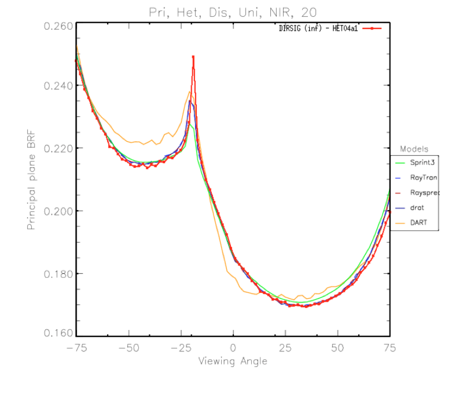
The following examples are based on scenes published by the RAdiation Model Intercomparision (RAMI) project which have published results for the bidirectional reflectance factor (limited to the principal and cross planes).

The active submission period for the "actual" canopies portion of RAMI IV (i.e. tree geometry with actual leaves/needles, branches, etc.. and designed to mimic measured sites) took place between 2009 and 2010, but no results have been published to date for these cases. This means that the verification process is limited to abstract canopy cases, some of which we present here.

Unless otherwise noted, all scene images are linked from http://rami-benchmark.jrc.ec.europa.eu

Real-Zoom Test Case (RAMI III)

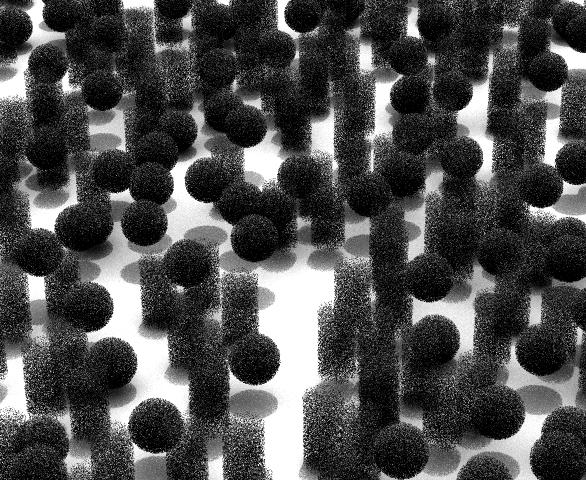
The Real-Zoom case describes a hetergeneous canopy with two (abstract) tree types. The trees are composed purely of leaf objects (no branches or trunks) which are modeled as disks with 5cm radii and distributed in either a sphere or cylinder shape. The BRFs for this scene are calculated for both the entire scene as well as smaller sections, though we only discuss the primary solution here.

Geometry

The coordinate system (corresponding to supplied data) is setup with the X axis pointing North and the Y axis pointing West, with the entire canopy enclosed within a 270 x 270 x 15m box.

The distribution of scatterers within each of the two "trees" is fixed with 31999 leaves in the spheres and 17999 leaves in the cylinders. We can translate the given list of disk centers and normals into DIRSIG primitives, such as the ODB file included in the example where the individual disks look like:

DISK {
    CENTER=2.969,-0.734,-1.122
    NORMAL=-0.224,-0.387,0.894
    RADIUS=0.05
    MATERIAL_ID=2000
}
DISK {
    CENTER=1.604,-3.212,-1.47
    NORMAL=0.943,0.106,0.316
    RADIUS=0.05
    MATERIAL_ID=2000
}
DISK {
    CENTER=1.637,-2.102,2.279
    ...

where we have translated the disk info given in the RAMI coordinate system (NWU) to the DIRSIG coordinate system (ENU).

An ODB (object data base) formatted file has been used here for brevity, though a glist (geometry list) could be used as well.

The list of disk instances for each tree in the scene is given in a scene level geometry list by including data in another file (this separation allows us to leave the glist alone while potentially updating generated data for the spheres and cylinders independently):

  <!-- SPHERES -->

  <object enabled="true">

    <basegeometry>
      <odb>
        <filename>leaves/sph.odb</filename>
      </odb>
    </basegeometry>

    <xi:include href="spheres.instances"/>

  </object>


  <!-- CYLINDERS -->

  <object enabled="true">

    <basegeometry>
      <odb>
        <filename>leaves/cyl.odb</filename>
      </odb>
    </basegeometry>

    <xi:include href="cylinders.instances"/>

  </object>

The included files just have lists of raw instances, for instance the "spheres.instances" file looks like:

<staticinstance><translation><point><x>-22.2713</x><y>-32.3813</y><z>5.6224</z></point></translation></staticinstance>
<staticinstance><translation><point><x>17.2922</x><y>-96.342</y><z>5.45672</z></point></translation></staticinstance>
<staticinstance><translation><point><x>-27.2434</x><y>-60.637</y><z>6.3866</z></point></translation></staticinstance>
<staticinstance><translation><point><x>-88.4261</x><y>87.0249</y><z>4.56644</z></point></translation></staticinstance>
<staticinstance><translation><point><x>-65.7388</x><y>120.93</y><z>9.57705</z></point></translation></staticinstance>
<staticinstance><translation><point><x>-18.0074</x><y>113.771</y><z>5.50713</z></point></translation></staticinstance>

which was generated by a short script that translated the provided instance locations from the scene information.

The rest of the scene consists of a simple (flat) ground plane.

Materials

The scatterers in the scene (disk "leaves") are assigned the given reflectances and transmittances and use the geodensity solver previously described. The sphere material, for instance, looks like:

MATERIAL_ENTRY {
    ID           = 2000
    NAME         = SPHERE LEAVES
    EDITOR_COLOR = 0.1, 0.1, 0.1

    RAD_SOLVER_NAME = GeoDensity
    RAD_SOLVER {
        MAX_BOUNCES = 100
        LOWER_EXTENT = -135, -135, -15
        UPPER_EXTENT =  135,  135, 0
        PADDING = 0
        TOP_ONLY = TRUE
        DIRECT_ONLY = FALSE
        DISABLE_DIRECT = FALSE
        CYCLIC_BOUNDARY = TRUE
        SOURCE_BUNDLES = 5e7
        SAVE_FILENAME = geoSph5e7b100.sav
        LOAD_FILENAME = geoSph5e7b100.sav

    }

    SURFACE_PROPERTIES {

        REFLECTANCE_PROP_NAME = WardBRDF
        REFLECTANCE_PROP {
            XY_SIGMAS  = 0, 0
            DS_WEIGHTS = 0.49, 0
        }

        TRANSMITTANCE_PROP_NAME = SimpleTransmission
        TRANSMITTANCE_PROP {
            FILENAME = leaf_sph.tau
        }
    }

    DOUBLE_SIDED = TRUE
}

Note that its important that the DOUBLE_SIDED property is set to true, otherwise rays and photon bundles hitting the backside will go write through it (this mechanism is used as an optimization for objects that don’t expose the backside of their surface). The reflectance is modeled as a purely diffuse reflectance (using a simple (monochromatic) version of the Ward BRDF model) and the transmittance is treated similarly (purely diffuse transmission), but with the total transmission set in a separate file. As suggested previously, we have the MAX_BOUNCES set to 100, though less than fifty successive scatterings take place for high fidelity runs and we have used a cyclic boundary with photon bundles being shot through the top only. The cylinder leaves are setup similarly, but with differences in the reflectance/transmittance.

Currently the geodensity maps for two different materials are built independently — this may change in the near future to cut down on the run time (the maps would be filled simultaneously).

The other materials in the scene, the ground (a diffuse reflector assigned the generic rad solver) and the portal materials (which give the translations to use when hit), are setup as well.

Generating Data

The other components of the scene setup as described previously or using standard types of inputs. In order to actually generate the results we can use the command line mode of running dirsig (rather than creating tasks and simulation files):

$ dirsig \
    --scene_filename=./scenes/UNI_NIR.scene \
    --atm_filename=./atm/BRF_20.atm \
    --platform_filename=./instruments/BRF_scripted.platform \
    --motion_filename=./instruments/BRF_scripted.ppd \
    --datetime="2013-06-21T12:00:00.0000+00:00"

The time of day is inconsequential (we fixed the solar ephemeris and there are no time dependent components to the scene). The resulting image (our 76 angular radiance samples) are written to an ENVI image file in the output directory.

In order to quickly extract data from the image we can use the image_analyze tool that is shipped with DIRSIG. Specifically we can extract all the data in the image by running:

$ image_analyze --image=<image filename> --operator=extract --band=0 > data.txt

which will generate a text file with the data (data is index in the file by sample and line position in the image). Note that the line index corresponds to the zenith angle, where 0 is the -75 degree measurement and the angle increases in 2 degree increments.

Selected Results

Figure 7. Verification with the RAMI Real-Zoom NIR principal plane BRF data for a source at 20 degrees. Results shown are for using a maximum of 100 scattering events (efffectively allowing the photon bundles to bounce to extinction).

Figure 8. Visualization of the spatial variation in the radiance collected for the previous BRF data plot. The bright flash about a third of the way through corresponds to the characteristic retroreflection of the source at 20 degrees (the peak seen in the plot). The apparent spatial distortion of the scene geometry is due to the constant area collection under varying angles.

Scene Download

RAMI3_DET_UNI.tgz